With the development of technology and industry, acoustic technology has become increasingly mature and is now widely used in areas ranging from consumer electronics to aerospace, and from medical facilities to scientific research. In various industrial inspection scenarios, equipment maintenance, and fault diagnosis, acoustic imaging has become a fast and convenient tool. It can transform sound waves that are difficult for the human ear to detect into intuitive images, helping technicians quickly locate problems. CRYSOUND’s Acoustic Imaging products are designed for partial discharge detection, gas leak detection, mechanical fault detection, and more, and have been widely adopted in over ten industries, such as power distribution, automotive, and composites. So, how exactly do acoustic imaging systems work? This blog will explain the complete workflow of an acoustic imaging system—from sound wave acquisition to visual imaging—in a simple and easy-to-understand way. CRYSOUND Acoustic Imaging Camera Products 1. Sound Wave Acquisition: Capturing Invisible Sound Waves The core function of an acoustic imaging system is to capture sound waves, which are usually generated by vibrations, leaks, or malfunctions during equipment operation. When sound waves propagate through the air, they cause air molecules to vibrate, forming pressure waves. Acoustic imaging systems receive these pressure waves through a built-in microphone array (usually composed of multiple high-sensitivity microphones). Each microphone can independently capture the frequency, intensity, and phase information of the sound wave, like taking a 'fingerprint' of the sound. For example, when a motor malfunctions, the wear of its internal bearings generates high-frequency vibrations. These vibrations propagate through the air and are captured by the microphone array of the acoustic imaging system. By analyzing these acoustic signals, technicians can initially determine the type and location of the fault. Gas Leak Detection Mechanical Faults Detection Partial Discharge Detection 2. Signal Processing: From Raw Data to Useful Information The acquired acoustic signals are analog signals and need to be converted into digital signals by an analog-to-digital converter (ADC). These digital signals then enter the signal processing unit for a series of complex calculations. These calculations include: Noise Reduction: Using digital filtering techniques, environmental noise and other interference signals are removed, retaining useful acoustic information. Beamforming: Utilizing the spatial distribution of the microphone array, algorithms calculate the direction and distance of the sound source. This process is similar to using multiple ears to locate the sound source. Spectrum Analysis: The acoustic signal is decomposed into components of different frequencies, and the intensity of each frequency component is analyzed to determine the nature of the sound source (e.g., mechanical faults, leaks, etc.). After these processes, the raw acoustic signal is transformed into useful information containing the sound source’s location, intensity, and frequency characteristics. 3. Visual Imaging: Converting Sound into Images The processed acoustic data needs to be presented to the user in an intuitive way. Acoustic imaging cameras visualize sound through the following steps: Data Mapping: Mapping the location information of the sound source onto two-dimensional or three-dimensional space to form a sound source distribution map. Typically, an acoustic imaging camera uses color to represent sound wave intensity: red or yellow indicates a strong sound source, and blue or green indicates a weak sound source. Image Overlay: Overlaying the sound source distribution map with a visible-light image or infrared image to form a composite image. This allows users to see the physical appearance of the equipment and the distribution of sound sources on the same image, thus quickly locating problem areas. Real-time Display: Acoustic imaging cameras typically provide real-time imaging capabilities, dynamically displaying changes in sound sources. This is extremely useful for monitoring equipment operating status and diagnosing faults. 4. Application Scenarios: A Wide Range of Uses The working principle of acoustic imaging makes it widely applicable in multiple fields. In the industrial field, acoustic imaging cameras can be used to detect mechanical faults, gas leaks, and electrical problems in equipment. For example, by analyzing the sound waves of a transformer during operation, it is possible to determine whether there is internal discharge or loosening. 5. Technical Advantages: High Efficiency, Precision, and Non-Contact The working principle of acoustic imaging systems gives them the following technical advantages: High Efficiency: Acoustic imaging cameras can quickly scan large areas and display the distribution of sound sources in real time, greatly improving detection efficiency. Precision: Through advanced signal processing algorithms, acoustic imaging cameras can accurately locate the position and intensity of sound sources, with errors typically within a few centimeters. Non-Contact: Acoustic imaging cameras do not require contact with the device under test, avoiding potential damage or interference from traditional detection methods. Conclusion Acoustic imaging systems transform invisible sound into intuitive images by capturing sound waves, processing signals, and visualizing images, providing a powerful tool for fault diagnosis and equipment maintenance. Although their working principle involves complex signal processing algorithms, the core logic is simple and easy to understand: from sound wave acquisition to visual imaging, every step is aimed at converting sound into useful information. With the continuous development of technology, acoustic imaging technology will continue to demonstrate its unique value in more fields. If you are interested in CRYSOUND’s acoustic imaging solutions or would like to discuss your specific application, please fill out the 'Get in touch' form below and our team will be happy to assist you.

For a long time, many engineers have seen sound calibrators as nothing more than little boxes that output 1 kHz at 94 dB: single-function devices, sensitive to the environment, not particularly pleasant to use in the field—yet still an indispensable link in any acoustic measurement chain. CRYSOUND’s all-new CRY3018 Sound Calibrator is designed to break this “good enough” mentality and upgrade sound level calibration from a passive, basic tool into an intelligent, reliable, and future-ready measurement reference. A Class 1 Smart Calibrator Built for the Field CRY3018 is a portable, high-precision sound calibrator fully compliant with IEC 60942:2017 Class 1. It can serve as a unified calibration reference in laboratories, on production lines, and in field measurements. Its core capabilities can be summed up in four key phrases: Dual-frequency calibration: 250 Hz / 1000 Hz Dual sound pressure levels (SPL): 94 dB / 114 dB Closed-loop SPL feedback with environmental self-compensation Intelligent power management with high-brightness OLED status display If traditional calibrators are still stuck in the era of fixed-level outputs, the CRY3018 is more like an intelligent calibration platform: it senses the environment in real time and compensates automatically. That’s where its truly disruptive value lies. Dual Frequencies + Dual Levels: One Device, More Scenarios In real-world work, a single 1 kHz, 94 dB calibration simply doesn’t cover all scenarios. Some standards or devices require calibration at 250 Hz. In noisy environments, a higher SPL is needed to secure enough signal-to-noise ratio. CRY3018 tackles all of these needs in one go: 250 Hz / 1000 Hz dual-frequency calibration: Meets different standards and device requirements for calibration frequency, better reflects the actual measurement bandwidth, and makes it easier to verify system frequency response more comprehensively. 94 dB / 114 dB dual SPL levels: 94 dB covers sensitivity calibration of conventional sound level meters and measurement microphones, while 114 dB effectively cuts through background noise in high-noise environments, ensuring the calibration signal stands out clearly. Typical performance figures include: Frequency accuracy: < 0.5 Hz SPL accuracy: < 0.2 dB THD+N: < 1% This means engineers no longer need to carry multiple calibrators with different frequencies and levels. One CRY3018 is enough to cover the vast majority of professional acoustic applications. Closed-Loop SPL Feedback + Environmental Three-Parameter Compensation: From “Rule-of-Thumb” Calibration to Self-Adaptive Calibration A major pain point of traditional calibrators is their extreme sensitivity to environmental changes. Even small shifts in temperature, humidity, or atmospheric pressure can introduce significant systematic errors—errors that historically have been estimated based on experience, or simply ignored. CRY3018 takes a fundamentally different architectural approach: Built-in SPL feedback system: It continuously monitors the actual sound pressure in the cavity and forms a closed control loop. If the output drifts, the system automatically adjusts to keep the SPL stable. Integrated high-precision temperature, humidity, and pressure sensors: These track three key environmental factors in real time. Combined with intelligent algorithms, the calibrator performs environmental self-compensation, effectively suppressing systematic deviations caused by environmental changes. In simple terms: Before: The environment changed, so humans had to worry and estimate. Now: The environment changes; the calibrator senses it and compensates automatically. This not only improves consistency and repeatability of measurement results, it also marks a genuine step into an environment-aware, data-driven smart calibration era—upending traditional workflows that relied heavily on experience and manual corrections. Intelligent Power Management: 5-Minute Fast Charge, Up to 1,000 Calibrations One of the worst nightmares for field engineers is this: “You’re ready to calibrate, and the calibrator is dead.” CRY3018’s power system is carefully engineered to avoid exactly that: USB-C fast charging with pass-through support (charge and use at the same time) About 5 minutes of quick charge provides roughly 1 hour of operation A full charge can support close to 1,000 calibration cycles On top of that, it integrates comprehensive safety and status management: Overcharge, over-discharge, and short-circuit protection Low-battery warning Auto power-on when a microphone is inserted, and auto power-off when removed In busy production lines or time-critical field tasks, CRY3018 can operate with minimal interruption, dramatically reducing the risk of interrupted testing due to power issues. Industrial Design and UX for Frontline Engineers CRY3018 is not just about stacking numbers on a spec sheet. Its emphasis on ergonomics and readability reflects a new product philosophy: Lightweight, high-strength carbon-fiber composite housing: Strikes a balance between weight and robustness; impact-resistant and scratch-resistant, comfortable for long periods of handheld use and frequent transport. High-brightness OLED display + auto-rotate via gyroscope: Whether you hold it vertically or horizontally, the screen automatically rotates to match the orientation. Readings remain clear in bright labs and outdoor environments. Top status LED + simple, intuitive button logic: White flashing: adjusting SPL Green solid: SPL stable and ready to use Red solid: low battery, shutting down soon While charging: yellow flashing; full charge: green solid Paired with intuitive interactions like short press to power on, long press to power off, and dedicated Hz / dB buttons to switch frequency and level, even first-time users can operate CRY3018 confidently without reaching for the manual. Full-Size Microphone Compatibility: A Unified Solution from Lab to Line CRY3018 supports 1" measurement microphones and, through adapters, is compatible with 1/2", 1/4", and 1/8" sizes, enabling: Laboratory-grade measurement microphone calibration Sound level meter calibration for environmental noise monitoring systems Sensitivity consistency checks for sensors on production lines Routine verification of acoustic test systems (audio analyzer + microphone arrays) For teams managing multiple microphone sizes and numerous test points, CRY3018 can act as a unified acoustic reference source, consolidating fragmented calibration workflows, reducing device variety, and simplifying management in a big way. More Than a Spec Upgrade: Rethinking How We Do Acoustic Calibration If you only look at the specs, CRY3018 is a leading, feature-rich Class 1 sound calibrator. But if you look at the entire workflow, it represents a new mindset: Calibration is no longer a check-the-box formality, but a smart, quantifiable, and traceable process. The environment is no longer an uncontrollable factor, but a parameter that can be sensed and compensated in real time. The calibrator is no longer a fixed-level box, but a unified reference platform that spans lab, field, and production line. What CRY3018 brings is not just a new generation of product—it’s a new answer to the question: What should acoustic calibration look like today? If your team is looking for a sound calibrator that truly fits both current and future measurement needs, the CRY3018 may be a strong starting point to redefine your entire calibration experience.

Electric motors are widely used in modern automobiles and home appliances (such as in-vehicle electric seats and appliance fans), and their smooth operation directly affects product quality and user experience. Motor noise issues are often summarized as BSR (Buzz, Squeak, and Rattle), which refers to abnormal sounds generated by automotive motors and related components. BSR has been a long-standing issue in manufacturing. It not only lowers the perceived quality of the product but also may signal problems such as bearing wear, loose parts, and other faults. Allowing defective products to reach the market can seriously damage brand reputation and user experience. Traditional "Manual Listening": Painful and Unreliable In the past, BSR detection usually relied on "manual listening," but human hearing has significant limitations: Subjective Misjudgment: When BSR noise is masked by background noise, the human ear cannot easily identify it. Judgments are based on experience, and results lack objective support. Unable to Quantify Analysis: The severity of BSR is difficult to quantify, making it difficult to establish clear quality standards. Low Efficiency and Fatigue: After prolonged testing, the human ear becomes fatigued, and detection accuracy declines, increasing the risk of defective products slipping through. Breaking the Bottleneck: Intelligent Solutions to Overcome Manual Limitations CRYSOUND, deeply rooted in the field of acoustic testing, has launched a BSR-based end-of-line (EoL) acoustic test solution for electric motors. By combining hardware, software, and AI, CRYSOUND has created a closed-loop testing process that gives motor abnormal sound detection an intelligent upgrade. Core Components: BSR Detection Hardware System + Testing Software Platform Soundproof Chamber: Creates a controlled, low-noise testing environment, blocking external noise that could disrupt BSR detection. Data Acquisition Module: Accurately captures sound and vibration data from the motor during operation, ensuring that even subtle anomalies are not overlooked. Algorithm Analysis: Processes, analyzes, and intelligently evaluates the captured signals, making BSR defects difficult to hide. Test Workflow: From Signal Capture to Intelligent Decision 1. First, sensors precisely capture sound and vibration signals, converting the sound of the motor into digital data. 2. Then, the system processes the data and automatically generates visual analysis results, clearly showing where abnormalities occur and how severe they are. 3. Finally, professional algorithms such as transient analysis, FFT spectrum analysis, and sound-quality evaluation are applied. With deep learning models, the system can automatically identify BSR caused by bearing wear, looseness, foreign-object interference, and other factors, greatly reducing human misjudgment and accurately separating good products from defective ones. Multi-Scenario Coverage: From Motors to High-End Manufacturing, Boosting Quality Control Across Industries This solution has been widely applied in the following areas: Motor Assemblies: BSR detection for various micro motors, drive motors, actuators, and other motor-related components. Automotive Parts: In the body domain—air-conditioning vents, seat systems/rails/motors, electric door handles, and other components; in the cockpit domain—HUD motors, display rotation mechanisms, electric sunroofs, and related parts; in the chassis domain—braking systems, steering systems, and associated components; in the autonomous driving domain—LiDAR modules and other systems requiring BSR evaluation. Home Appliances: BSR detection for motors and motorized components used in high-end household appliances and smart home devices. Others: Industrial scenarios requiring stringent sound quality assessment and high-precision BSR detection. Five Major Advantages: Making Quality Inspection Smarter AI Acoustic Detection: By replacing manual inspection with machines, detection becomes more objective and efficient and supports continuous, high-throughput operation in production environments. Accurate BSR Capture and Visual Presentation: The characteristics of BSR are visually displayed through data charts, making problems easy to identify at a glance. Supports Full EoL Testing, Traceable Results: All process data is retained, making quality traceability clear and compliant with regulations. Highly Integrated One-Stop Solution, Improved Production Efficiency: This highly integrated, one-stop solution streamlines the testing process and seamlessly connects to the production line, enhancing overall production efficiency. Helps Improve Yield and Reduce Customer Complaints: Ensures strict quality control, making it difficult for defective products to leave the factory and significantly reducing customer complaints. If you are interested in CRYSOUND's intelligent BSR noise detection solution or would like to discuss your specific testing needs, please fill out the "Get in touch" form below and our team will be happy to assist you.

In acoustic and vibration testing, engineering teams often find themselves jumping between multiple software tools and data acquisition systems from different vendors. Interfaces vary, workflows are fragmented, and new engineers can spend a significant amount of time just learning the tools before they can focus on the engineering problem itself. OpenTest, developed by CRYSOUND, is a next-generation acoustic and NVH testing platform designed for engineers, researchers, and manufacturers. Built around the principles of an open ecosystem, AI-driven intelligence, and high compatibility, it allows users to complete the entire workflow—from acquisition to reporting—within a single software environment. OpenTest supports three operating modes: Measure, Analysis, and Sequence, covering both laboratory validation and repetitive production testing. Core capabilities include real-time monitoring and analysis, FFT and octave analysis, sweep analysis, sound power testing, sound level meter functions, and sound quality analysis. The platform also provides standard test reports and dedicated sound power reports that comply with international standards. On the hardware side, OpenTest connects to a wide range of multi-brand DAQ devices via mainstream audio protocols such as openDAQ, ASIO, and WASAPI, as well as optional proprietary drivers such as NI-DAQmx, enabling unified management of CRYSOUND SonoDAQ, RME, NI, and other devices within a single platform. On the software side, its modular plugin architecture exposes interfaces for Python, MATLAB, LabVIEW, C++ and more, making it easy for teams to package in-house algorithms and domain applications as plugins and deploy them within the same environment. From Acquisition to Report: A Three-Step Quick-Start Workflow 1. Installation and Basic Connectivity – Let the Signals In Download the latest installer from the official website www.opentest.com and complete the installation. Connect your DAQ device to the PC; for your first trial, you can simply use the built-in PC sound card to run a quick test. In the OpenTest setup section, scan for available devices and select the devices and channels you want to use. Once added to the project, your basic connectivity is complete. 2. Run Basic Tests with Real-Time Analysis – See It First, Then Optimize In the channel management view, select the input/output channels you want to use and configure key parameters such as sensitivity, sampling rate, and gain. The system automatically activates the Monitor panel, where you can view real-time waveforms, FFT spectra, and key metrics such as RMS level and THD at a glance. When needed, you can enable the built-in signal generator to output excitation signals and use the recording function for long-duration acquisition, preserving data for later comparison and analysis. 3. Perform In-Depth Analysis and Reporting in the Measure Module – Turning Data into Decisions Switch to the Measure module to access advanced applications such as FFT analysis, octave analysis, sweep analysis, sound power testing, sound level meter, and sound quality—providing everything you need for deeper investigation. Use the data set functionality to review and overlay historical records, so you can compare different samples, operating conditions, or tuning strategies side by side. Waveforms and analysis results can be exported at any time. With the reporting function, you can generate test reports with a single click, closing the loop from test execution to final deliverables. Who Is OpenTest For? New acoustic and vibration test engineers who want to establish a complete workflow quickly using a single toolchain. Laboratories and corporate teams that need to manage multi-brand hardware and consolidate everything into one unified software platform. Project teams in automotive NVH, consumer electronics, and industrial diagnostics that require high channel counts, automation, and AI-enhanced analysis capabilities. Wherever you are on your testing infrastructure journey, OpenTest lets you start with a free entry-level edition and adopt an open, intelligent, and scalable ecosystem with a low barrier to entry. Visit www.opentest.com to explore detailed features, supported hardware, and licensing and plan options, and book a demo to see how OpenTest and CRYSOUND can help you build an efficient, open, and future-ready acoustic and vibration testing platform.

The all-new OpenTest website (opentest.com) is live, bringing product capabilities, ecosystem, docs, updates, and download into a single, streamlined experience to help engineers, researchers, and manufacturers get productive fast. At a Glance Clear information architecture with top-level navigation to Features / Hardware / Plugin / Pricing / About / Docs / Updates / Download. Three work modes tailored to real workflows: Measure, Analysis, Sequence. Feature matrix in one view covering Monitor, FFT, Octave, Sweep, Sound Power, Export/Report. Open ecosystem for hardware and plugins, supporting mainstream audio/DAQ interfaces and multiple development languages. Transparent plans with Community, Professional, and Enterprise options. Bulit for Engineers Three Work Modes Measure Mode — Real-time acquisition with live metrics plus post-run analysis for flexible review. Analysis Mode — Deep, offline analysis from data cleaning to computation. Sequence Mode — Purpose-built for repetitive/production tests, integrating acquisition → analysis → storage → reporting for repeatable throughput. Key Capabilities Monitor, FFT, Octave, Sweep, Sound Power, Export, and Report—covering mainstream acoustic and vibration analysis in lab or line environments. Open Ecosystem: Hardware & Plugins Open Hardware Access Protocol with compatibility for openDAQ, ASIO, WASAPI (and optional private protocols such as NI-DAQmx) to connect a wide range of DAQ devices. Three-layer plugin architecture — Algorithm / Theme / Application — enabling full-stack extensibility. Develop with Python, MATLAB, LabVIEW, C++, and more. Open-Source Core + Commercial Capabilities CommunityFully open-source core functions; 2 channels; Algorithm plugins; built-in Monitor/FFT/Octave/Basic Sweep/General Report; community forum support. ProfessionalUp to 24 channels; Algorithm + Theme plugins; Advanced Sweep and Sound Power; email support. EnterpriseUnlimited channels; Algorithm + Theme + Application plugins; white-label options and customization; enterprise-grade support and compliance. Get Started in Seconds Download for Windows from the homepage. The relaunch brings open ecosystem + clear capability boundaries + transparent plans onto one page—smoothing both decision-making and deployment. If you’re building or upgrading an acoustic/NVH testing platform, start with the new site, pick a plan, download, and close the loop from acquisition to reporting—faster.

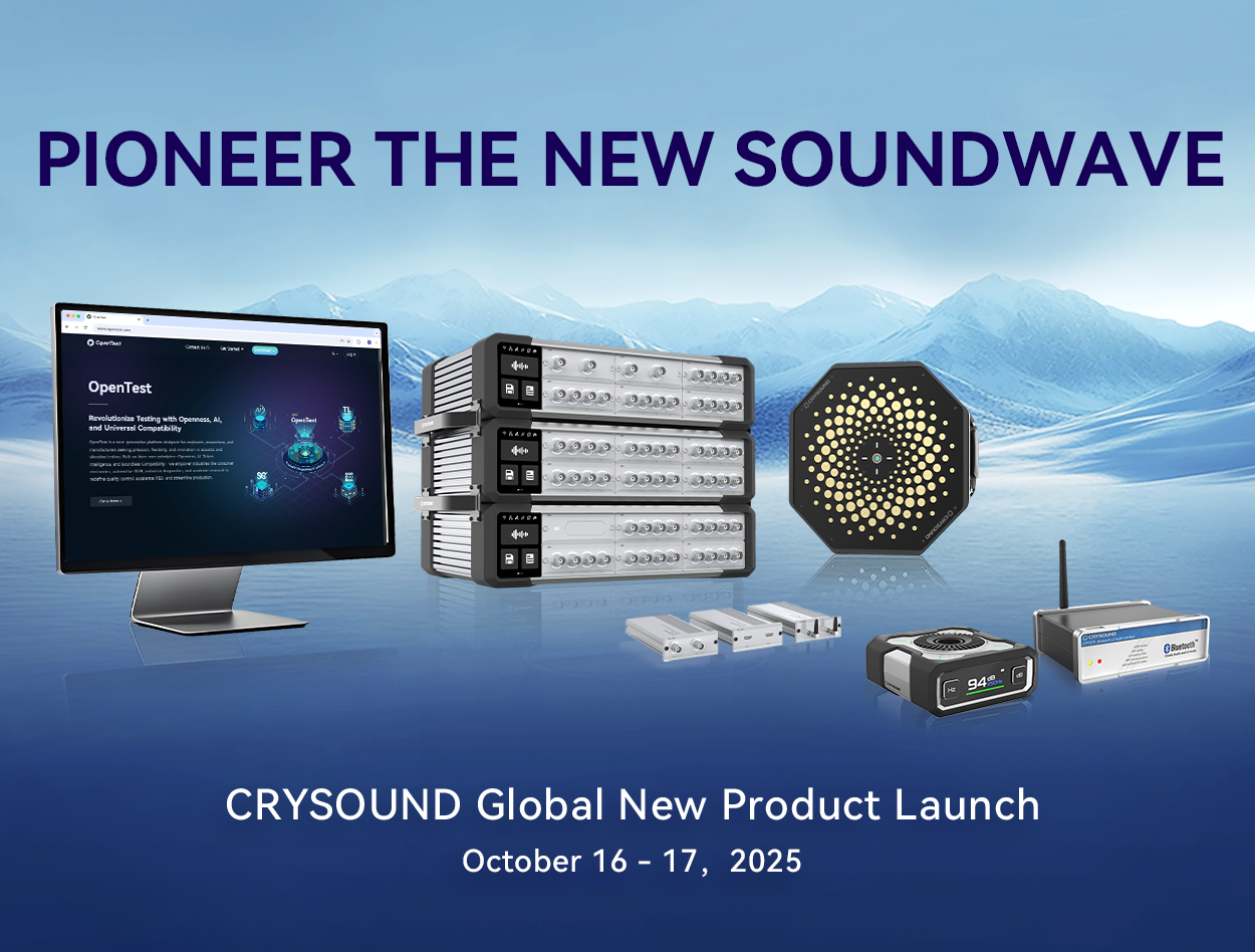
On October 16–17, 2025, the CRYSOUND Global New Product Launch 2025 successfully took place in Hangzhou. The conference showcased the company’s latest innovations across multiple key areas, such as data acquisition, acoustic imaging, sound calibration, and Bluetooth audio. Newly launched products include SonoDAQ, OpenTest, the CRY8500 Series SonoCam Pi Acoustic Camera, the CRY3010 Series Sound Calibrator, and the CRY578 Bluetooth LE Audio Interface. During the conference, customers, partners, and industry experts from more than twenty countries gathered to explore cutting-edge innovations and future applications in acoustic technology. New Product Highlights On October 16, CRYSOUND officially launched five new products — SonoDAQ, OpenTest, CRY8500 Series SonoCam Pi Acoustic Camera, CRY3010 Series Sound Calibrator, and CRY578 Bluetooth LE Audio Interface. These latest innovations embody CRYSOUND’s continuous pursuit of excellence, delivering advanced performance, reliability, and flexibility for acoustic testing and measurement. SonoDAQ – Next-Generation Data Acquisition Hardware High Performance SonoDAQ uses PTP and GPS synchronization with inter-device latency under 100 ns, ensuring unified timing across all channels. With 1000 V isolation and a dual-gain, dual-ADC design, it delivers a 170 dB dynamic range for accurate, stable acquisition. High Reliability SonoDAQ features a rubber–carbon fiber–aluminum composite structure. Its chassis is precision-formed under 5,000 tons of pressure, withstanding the weight of two cars without performance loss. The unique T-shaped aluminum extrusion increases the heat dissipation area by 35%, ensuring long-term stability even in harsh environments. High Flexibility Offers USB-C, CAN FD, GLAN interfaces and hot-swappable batteries. Five operating modes—standalone, offline recording, small-scale daisy-chain, distributed, and large-scale star-chain—expand to 1,000+ channels. Modular design saves space and simplifies expansion. High Scalability Fully compatible with openDAQ, ASIO, DAQmx, WASAPI, and integrates with MATLAB, LabVIEW, Python, C++, building an open, modular ecosystem. OpenTest – Next-Generation Software Modular Front-end and back-end are separated, with an open-source core. Algorithms, logic, and interface are clearly decoupled, ensuring stability, easy maintenance, and independent upgrades. Cross-Platform Built on a cross-platform framework, runs natively on Windows, macOS, and Linux, providing consistent high performance. Extensible Supports a three-layer plugin system—algorithms, themes, applications. Users can integrate custom logic using Python, C++, or other mainstream languages to create tailored workflows. Lightweight, High-Performance, Sustainable Designed with efficient libraries and a streamlined architecture, it starts quickly with low resource usage, ready to meet technological and business demands for the next decade. CRY8500 Series SonoCam Pi Acoustic Camera Customizable, Replaceable Microphone Arrays Modular design supports four array configurations: 30 cm 128-channel, 30 cm 208-channel, 70 cm 208-channel, 110 cm 208-channel, with up to 208 MEMS microphones. Far-Field Beamforming & Near-Field Acoustic Holography Supports both far-field beamforming and near-field acoustic holography, switchable on the device. Real-Time Data Output API Provides API for real-time waveform and video output of up to 208 channels. 500 m UAV Detection & Tracking The 30 cm 208-channel array enables real-time detection and tracking of drones within 500 m. Class 1 Frequency Response Compliant with sound level meter standards, ensuring Class 1 frequency accuracy. CRY3010 Series Sound Calibrator Easy to Use The calibrator supports four microphone sizes from 1″ to 1/8″ via adapters. Its built-in lithium battery provides up to 365 days of operation on a full charge, or about 30 days from a 5-minute top-up. The OLED display offers high brightness of 450 nits and features auto-rotate and auto power on/off. High Stability The calibrator provides dual-frequency operation at 250 Hz and 1000 Hz, and dual sound levels of 94 and 114 dB. Precision feedback microphones and sensors provide environmental compensation for temperature, humidity, and pressure. High Reliability The carbon-fiber composite housing with rubber enhances drop resistance. The sound-damping enclosure and precision digital filtering effectively suppress environmental noise, ensuring measurement accuracy and long-term reliability. CRY578 Bluetooth LE Audio Interface Advanced Bluetooth Technology Supports Bluetooth 5.4, both Classic Audio and LE Audio, with sample rates from 16 kHz to 96 kHz. Rich Interface Options Equipped with UAC, Line in/out, and S/PDIF in/out, seamlessly integrating with various test systems. Wide Compatibility Works with major Bluetooth chipsets and supports SBC, AAC, aptX, LHDC, LDAC, LC3, LC3 plus codecs for fast connection and efficient testing. Intelligent Software Management Includes CRY578 Tool for protocol configuration and real-time log analysis. On-site Product Showcase Next to the main venue, CRYSOUND set up ten booths to highlight both its latest innovations and classic products. The live demonstration of ten networked SonoDAQ units became a key attraction, featuring PTP precision synchronization with under 100 ns inter-device latency, modular expansion, and intelligent LED backplane indicators, fully showcasing the system’s high-precision distributed acquisition capabilities. In combination with the OpenTest platform, SonoDAQ also powered demonstrations of the Intelligent Electroacoustic Testing System and Sound Power Testing Solution, offering a seamless workflow from configuration and data acquisition to automated report generation, significantly improving the efficiency of multi-channel electroacoustic and acoustic testing. The atmosphere was lively, with acoustic industry experts, customers, and CRYSOUND engineers engaging in in-depth discussions on innovative testing applications and future developments. Factory and Showroom Visit Clients and industry experts visited the CRYSOUND factory and showroom. The factory showcased the company’s craftsmanship and strict quality control across all product lines, giving visitors an in-depth understanding of the professionalism and quality behind each product. The showroom highlighted CRYSOUND’s development history and comprehensive product portfolio. They also toured the new headquarters under construction, learning about its planned R&D and production layout and witnessing CRYSOUND’s commitment to advancing acoustic technology. Training Sessions On the morning of October 17, CRYSOUND held specialized training sessions on SonoDAQ and OpenTest. Engineers combined live demonstrations with hands-on practice, showcasing how the two systems work together and their applications in typical testing scenarios. The sessions provided clear, practical insights into system functions and workflows, earning positive feedback from all participants. Roundtable Discussion At the close of the conference, a roundtable discussion on “The Future of AI in Acoustic Measurement” brought the event to a successful conclusion. CRYSOUND CEO Jason Cao and five industry experts explored industry trends, technological innovations, and the application of AI in acoustic measurement, exchanging insights and experiences to generate valuable perspectives for the future development of the industry. The CRYSOUND Global New Product Launch 2025 not only unveiled the company’s latest innovations but also brought together industry leaders, partners, and customers from over twenty countries. Attendees experienced the impressive performance of five new products, explored the factory and showroom, and participated in hands-on training that reinforced confidence in CRYSOUND’s expertise. Expert speeches and the roundtable discussion offered fresh insights and sparked forward-looking ideas for the industry. Looking ahead, CRYSOUND will continue to drive innovation, strengthen global partnerships, and explore new frontiers in intelligent acoustics, delivering lasting value to the industry.

Hosted by the Acoustical Society of China and exclusively sponsored by CRYSOUND , the Final Round of the 3rd “Shenghua Cup”National Acoustic Technology Competition successfully concluded in Hangzhou on October 11, 2025. This year’s competition attracted 61 teams from 39 universities and research institutes across China. Young acoustic talents demonstrated the remarkable strength and creativity of China’s new generation of acoustic researchers through hands-on challenges. The practical testing session of this year's “Shenghua Cup” was designed around real-world acoustic measurement scenarios. Relying on CRYSOUND's self-developed zero-threshold development kit — SonoCam Pi, the competition comprehensively assessed the participants' overall capabilities in system setup, data acquisition, and algorithm implementation. Despite complex testing environments and technical challenges, the participants remained composed and collaborative, skillfully integrating theory with practice and demonstrating solid professional competence. During the academic defense session, expert judges evaluated and questioned the teams from multiple dimensions — including algorithmic logic, technical depth, and application value. The lively exchanges of ideas showcased both the rigorous scientific mindset and the innovative spirit of acoustic research. CRYSOUND also organized the “Exploring the World of Acoustic Technology” tour, opening its showroom and production lines to experts and student teams. Through guided explanations and live demonstrations by CRYSOUND engineers, visitors gained close-up insights into the company’s core products — such as Acoustic Imaging Cameras, SonoCam Pi, Data Acquisition Systems, Measurement Microphones, and Calibrators — and engaged in in-depth discussions on the industrialization pathways of acoustic technologies. As the exclusive sponsor and organizer of the event, CRYSOUND not only provided full hardware and technical support, but also offered participation subsidies to every student team, encouraging them to focus fully on hands-on experimentation in the anechoic chamber without concerns. Jason Cao, CEO of CRYSOUND, remarked: “We hope the ‘Shenghua Cup’ is more than just a competition — it serves as a bridge linking universities, research institutes, and industries. Through this event, many innovative ideas have gained recognition from the industry and even led to potential collaborations. This is the true meaning of ‘industry-academia-research integration.’” While the competition may have concluded, innovation never stops. CRYSOUND extends heartfelt thanks to the Acoustical Society of China, to every expert, teacher, and student for their dedication and passion. Looking ahead, CRYSOUND will continue to work with industry partners to build a more open and dynamic innovation platform, helping more acoustic technologies move from the laboratory to industrial applications — together shaping a brighter future for the field of acoustics.

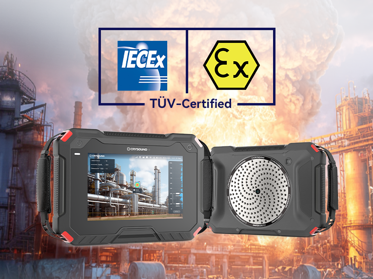
The industry's first TÜV-certified acoustic imaging camera with dual explosion protection (IECEx & ATEX), designed to redefine industrial inspection in hazardous environments. CRYSOUND proudly introduces the CRY8125 Ex Acoustic Imaging Camera — a cutting-edge solution specifically engineered for explosive atmospheres. With TÜV certification and full compliance with IECEx and ATEX Zone 2 standards, the CRY8125 Ex is purpose-built for reliable performance in hazardous environments. It combines advanced acoustic imaging capabilities such as gas leak detection, leak rate measurement, partial discharge detection and classification — setting a new benchmark for industrial inspection in explosive atmospheres. The Industry's First with TÜV-Certified Dual Explosion Protection The CRY8125 Ex Acoustic Imaging Camera is TÜV-certified for Zone 2 operation under both the IECEx and ATEX schemes, holding the following markings: II 3 G Ex ic IIC T5 Gc / II 3 D Ex ic IIIC T100°C Dc. It fully complies with IEC 60079-0 and IEC 60079-11 standards, ensuring safe and reliable use in potentially explosive gas and dust environments. This dual certification makes the CRY8125 ideal for hazardous-area applications in industries such as oil & gas, petrochemicals, chemicals, and gas-fired power generation, where explosion protection is mission-critical. Detect Any Type of Gas in Hazardous Zones The CRY8125 Ex Acoustic Imaging Camera is engineered to detect a wide variety of gases — including natural gas, hydrogen, carbon monoxide (CO), and volatile organic compounds — even in explosive environments such as refineries, chemical plants, and gas facilities. It provides: Real-time leak quantification Instant estimation of potential economic loss Actionable data for fast maintenance decisions Built to Withstand the Harshest ConditionsTo ensure reliable field performance, the CRY8125 undergoes 28 days of rigorous environmental testing, including: High-temperature aging at 90°C Low-temperature exposure at -25°C 90% humidity cycling Drop tests to verify durability After completing these extreme tests, the CRY8125 maintains its IP54 rating— ensuring consistent operation under demanding industrial conditions. High-Performance Intrinsically Safe Acoustic Imaging Camera The CRY8125 features 200 microphones, a 100 kHz bandwidth, and the fastest processor to detect smaller leaks and partial discharges at greater distances. It’s widely used in oil, natural gas, chemical, and gas power industries. Its 8-inch 2K display offers 2 million pixels, 6x digital zoom, and 600-nit brightness, ensuring clear imaging even in direct sunlight for detailed inspections. With an extended detection range, the CRY8125 improves test efficiency over 4× while keeping operators safe by minimizing exposure to toxic gases and covering a wider area. Comprehensive Hardware Configuration The CRY8125 is designed for versatility and future-proof expansion: Supports Bluetooth and Wi-Fi for seamless direct data transfer to local devices Accommodates up to 4 IEPE sensors (such as accelerometers and microphones) to enable advanced detection capabilities All-in-One Workflow: From Detection to Reporting The CRY8125 features an integrated workflow that streamlines the entire inspection process—from image capture and acoustic analysis to automatic report generation. This greatly enhances the efficiency of gas leak detection, allowing for quicker decision-making and safer, more reliable operations. Real-World Applications The CRY8125 enables safer and more efficient inspections across multiple industries. Oil Industry: Detect hazardous leaks such as H₂S, CH₄, and VOCs to eliminate safety risks Natural Gas: Monitor pipelines and storage tanks to detect leaks and prevent economic loss Chemical Industry: Non-contact detection of Cl₂, H₂, N₂, and steam ensures operational safety Gas Power Generation: Identify gas leaks in tanks and partial discharges in transformers quickly and effectively Case Studies: Field-Proven Performance A coal chemical enterprise successfully located a gas leak in an overhead pipeline that traditional methods failed to detect. At a natural gas storage station, the CRY8125 Ex identified 8 leak points in just one minute, dramatically improving inspection efficiency. Set a New Standard in Acoustic Imaging Safety With its dual explosion-proof certification, intelligent workflow, and proven durability, the CRY8125 Ex Acoustic Imaging Camera is an essential solution for modern industrial inspection in hazardous environments. Discover the future of acoustic inspection—safe, smart, and fast.To learn more or request a demo, please reach out to us at info@crysound.com.