

In our previous blog post, "Abnormal Noise Detection: From Human Ears to AI"we discussed the key pain points of manual listening, introduced CRYSOUND's AI-based abnormal-noise testing solution, outlined the training approach at a high level, and showed how the system can be deployed on a TWS production line. In this post, we take the next step: we'll dive deeper into the analysis principles behind CRYSOUND's AI abnormal-noise algorithm, share practical test setups and real-world performance, and wrap up with a complete configuration checklist you can use to plan or validate your own deployment.
Challenges Of Detecting Anomalies With Conventional Algorithms
In real factories, true defects are both rare and highly diverse, which makes it difficult to collect a comprehensive library of abnormal sound patterns for supervised training.
Even well-tuned-sometimes highly customized-rule-based algorithms rarely cover every abnormal signature. New defect modes, subtle variations, and shifting production conditions can fall outside predefined thresholds or feature templates, leading to missed detections (escapes).
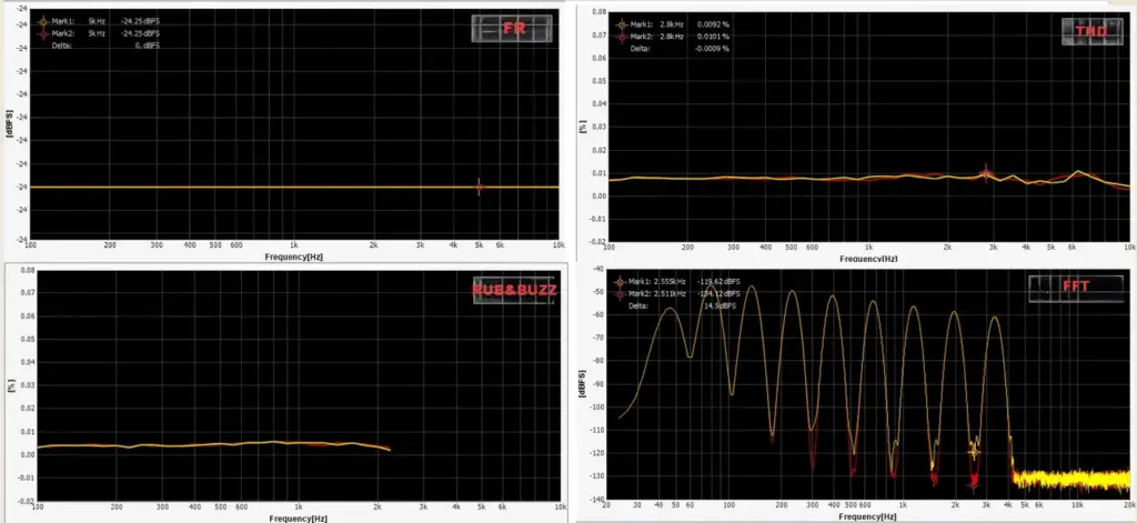
In the figure below, we compare two wav files that we generated manually.
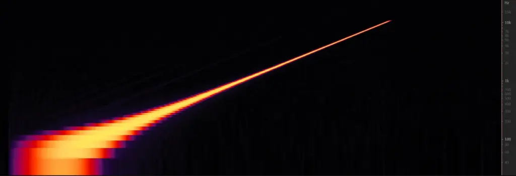
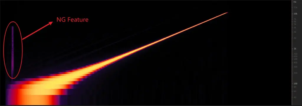
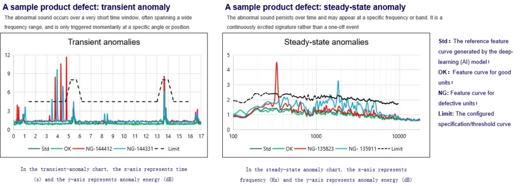
You can see that conventional checks-frequency response, THD, and a typical rub & buzz (R&B) algorithm-can hardly detect the injected low-level noise defect; the overall curve difference is only ~0.1 dB. In a simple FFT comparison, the two wav files do show some discrepancy, but in real production conditions the defect energy may be even lower, making it very likely to fall below fixed thresholds and slip through. By contrast, in the time-frequency representation , the abnormal signature is clearly visible, because it appears as a structured pattern over time rather than a small change in a single averaged curve.
Principle Of AI Abnormal Noise Algorithm
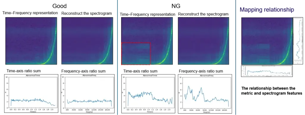
CRYSOUND proposes an abnormal-noise detection approach built on a deep-learning framework that identifies defects by reconstructing the spectrogram and measuring what cannot be well reconstructed. This breaks through key limitations of traditional rule-based methods and, at the principle level, enables broader and more systematic defect coverage-especially for subtle, diverse, and previously unseen abnormal signatures.
The figure below illustrates the core workflow behind our training and inference pipeline.

During model training, we build the algorithm following the workflow below.
How To Use And Deploy The AI Algorithm
Preparation
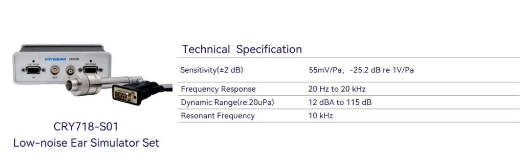
First, prepare a Low-Noise Measurement Microphone / Low-noise Ear Simulator and a Microphone Power Supply to ensure you can capture subtle abnormal signatures while providing stable power to the mic.
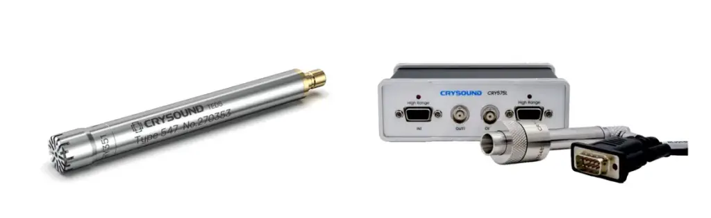
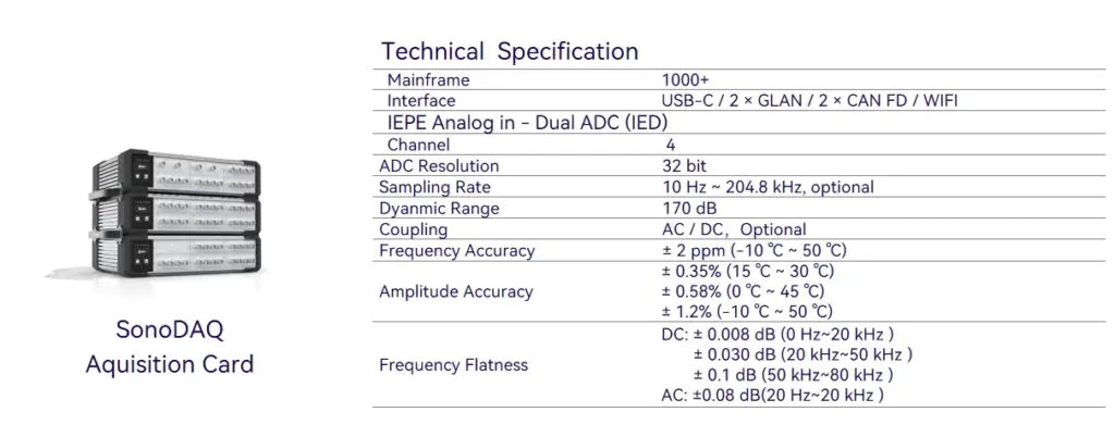
Next, you'll need a sound card to record the signal and upload the data to the host PC.

Third, use a fixture or positioning jig to hold the product so that placement is repeatable and every recording is taken under consistent conditions.
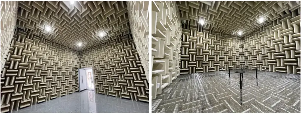
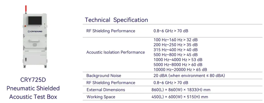
Finally, ensure a quiet and stable acoustic environment: in a lab, an anechoic chamber is ideal; on a production line, a sound-insulation box is typically used to control ambient noise and keep measurements consistent.

Model Development
First, create a test sequence in SonoLab, select "Deep Learning" and apply the setting.
Next, select the appropriate AI abnormal-noise algorithm module and its corresponding API
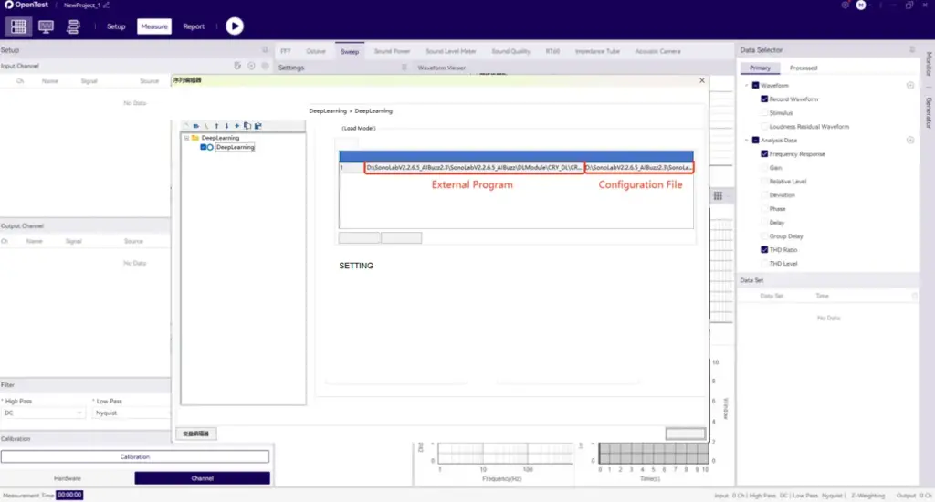
Then open Settings and specify the model type, as well as the file paths for the training dataset and test dataset.
Click Train and wait for the model to finish training (Training time depends on your PC's hardware)
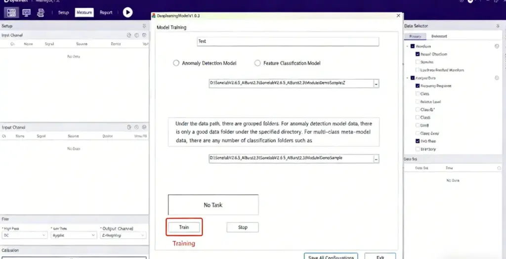
During training, the status indicator turns yellow. Once training is complete, it switches to green and shows a "Training completed" message.

Finally, place your test WAV files in the specified test folder and run the sequence. The model will start automatically and output the analysis results.
Test Case

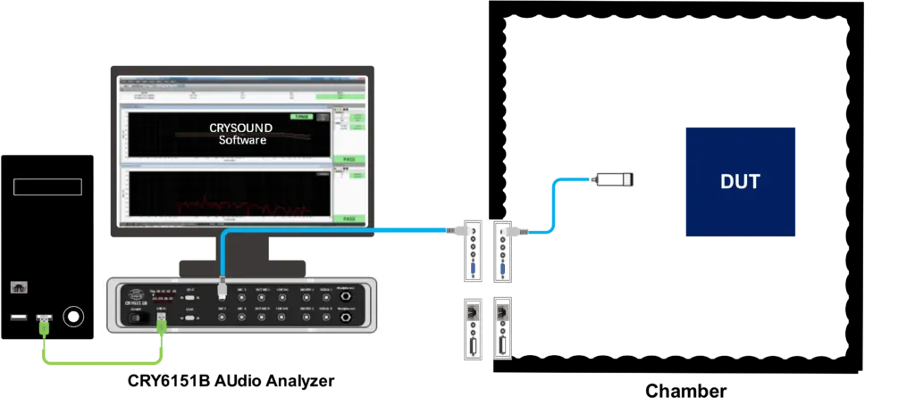
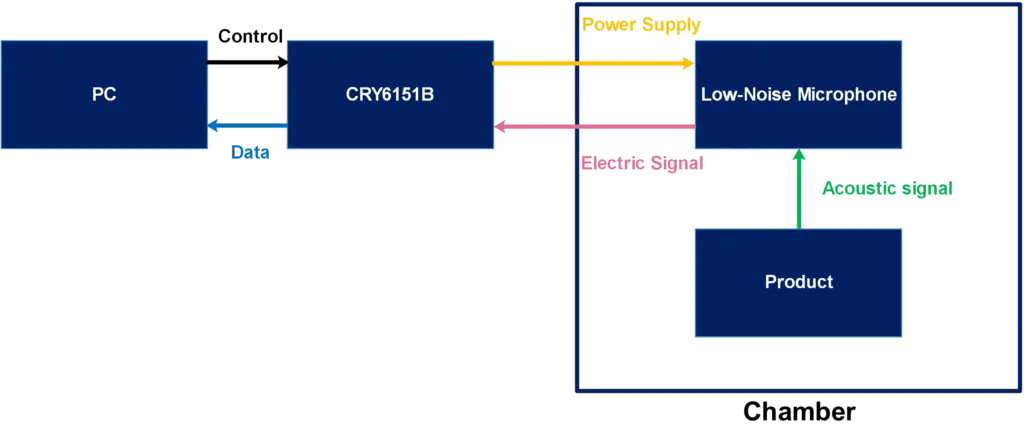
System Block Diagram
Equipment
More technical details are available upon request-please use the "Get in touch" form below. Our team can share recommended settings and an on-site workflow tailored to your production conditions.
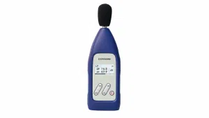
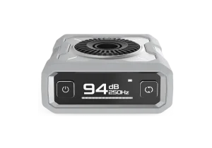
CRY2831 Class 2 Sound Level Meter

CRY8024 SonoCam Pocket Acoustic Camera
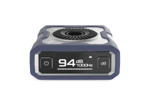
CRY3016 Sound Calibrator
CRY3012 Sound Calibrator
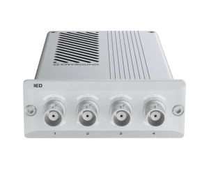
CRY5011 IEPE Analog In - IED
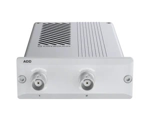
CRY5085 Analog Output Class D 10W - ADD
CRY2831 Class 2 Sound Level Meter
CRY8024 SonoCam Pocket Acoustic Camera
CRY3016 Sound Calibrator
CRY3012 Sound Calibrator
CRY5011 IEPE Analog In - IED
