Sound is everywhere in our daily life: birdsong, street noise, engine roar, even the faint airflow from an air conditioner. For people, sound is not only about whether we can hear it, but whether it feels comfortable, is disturbing, or poses a risk. The same 70 dB can feel completely different; and when something feels "noisy", the cause may come from the source itself, the propagation direction, or reflections from the environment. When we turn this "perception" into quantifiable engineering data, the three most easily confused concepts are sound pressure, sound intensity, and sound power. They answer: Sound pressure: how loud it is at a specific point; Sound intensity: how much sound energy is propagating in a particular direction; Sound power: how loud the source is in terms of its total acoustic emission; This article explains sound pressure, sound intensity, and sound power in an intuitive way, so you can better understand sound. Sound Waves In engineering acoustics, sound pressure, sound intensity, and sound power are three fundamental and important physical quantities. Before introducing them in detail, we need the concept of a sound wave. A vibrating source sets the surrounding air particles into vibration. The particles move away from their equilibrium position, drive adjacent particles, and those adjacent particles generate a restoring force that pushes the particles back toward equilibrium. This near-to-far propagation of particle motion through the medium is what we call a sound wave. Figure 1. Propagation of a Sound Wave in Air Sound Pressure When there is no sound wave in space, the atmospheric pressure is the static pressure p0. When a sound wave is present, a pressure fluctuation is superimposed on p0, producing a pressure fluctuation p1. Here p1 is the sound pressure (unit: Pa). Therefore, sound pressure is the instantaneous deviation of the air static pressure caused by the sound wave. The human brain does not respond to the instantaneous amplitude of sound pressure, but it does respond to the root-mean-square (RMS) value of a time-varying pressure. Therefore, the sound pressure p can be expressed as: In practical engineering applications, the sound pressure level Lp: where Pref = 2 × 10-5 Pa is the reference sound pressure. In practice, we usually use sound pressure level (dB) to characterize sound pressure, rather than using pressure in pascals. Why? Figure 2 answers this well. From a library to the entrance of a high-speed rail station, sound pressure may increase by a factor of 100, while sound pressure level increases by only 40 dB. This reflects the difference between a linear scale and a logarithmic scale. From an engineering perspective, using sound pressure directly leads to large numeric variations that are inconvenient for evaluation. Moreover, the human auditory system is closer to a logarithmic response, so sound pressure level better matches hearing. Figure 2. Sound Pressure and Sound Pressure Level Sound Intensity Sound intensity describes the transfer of acoustic energy. It is the acoustic power passing through a unit area per unit time. It is a vector quantity that is directional, with units of W/m2, defined as the time average of the product of sound pressure and particle velocity: where v(t) denotes the particle velocity vector. Under the ideal plane progressive-wave approximation, sound pressure and particle velocity approximately satisfy: where ρ is the air density, c is the speed of sound. Therefore, the magnitude of sound intensity along the propagation direction can be written as: Similarly, sound intensity has a corresponding intensity level LI: where I0 = 10-12 W/m2 is the reference sound intensity. Compared with sound pressure level measurements, sound intensity measurements have the following characteristics: Directional:it can distinguish whether acoustic energy is propagating outward or flowing back, so under typical field conditions it is often less sensitive to reflections and background noise; Source localization:intensity scanning can directly reveal the main radiation regions and leakage points, making remediation more targeted; Higher system complexity:it typically requires an intensity probe, with higher overall cost and more setup and calibration effort; Figure 3. Sound Intensity Testing A key advantage of sound intensity measurement in engineering applications is that it characterizes both the direction and magnitude of acoustic energy flow. It can separate the contributions of outward radiation from the source and reflected backflow from the environment, so under non-ideal field conditions it tends to be less affected by reflections and background noise. In addition, the sound intensity method can obtain sound power directly by spatially integrating the normal component of intensity over an enclosing surface. Combined with surface scanning, it can identify dominant source regions and locate leakage points. Therefore, it is highly practical and interpretable for noise diagnosis, verification of noise-control measures, and sound power evaluation. The key instrument for sound intensity testing is the sound intensity probe. Unlike a single microphone, an intensity probe is not used merely to measure “how large the pressure is”; it must provide the basic quantities required for calculating intensity (sound pressure and particle velocity). Therefore, the probe typically outputs two synchronous channels and, together with a two-channel data-acquisition front end and dedicated algorithms, yields intensity results. In engineering practice, the probe often includes interchangeable spacers, positioning fixtures, and windshields. Channel amplitude/phase matching, phase calibration capability, and airflow-interference mitigation directly determine the credibility and usable frequency range of intensity measurements. Two types of sound intensity probes are commonly used: P-U probes (pressure-particle-velocity) and P-P probes (pressure-pressure). A P-U probe consists of a microphone and a velocity sensor, measuring sound pressure p(t) and particle velocity v(t) simultaneously. The principle is more direct, but particle-velocity sensors are often more sensitive to airflow, contamination, and environmental conditions, requiring more protection and maintenance in the field and usually costing more. Figure 4. P-U Sound Intensity Probe (Microflown) A P-P probe uses two matched microphones aligned on the same axis. It uses the two pressure signals p1(t) and p2(t) to estimate the particle-velocity component v(t). However, it is sensitive to inter-channel phase matching and the choice of microphone spacing - the spacing determines the effective frequency range: a larger spacing benefits low frequencies, but high frequencies suffer from spatial sampling error; a smaller spacing benefits high frequencies, but low frequencies become more susceptible to phase mismatch and noise. Figure 5. P-P Sound Intensity Probe (GRAS) P-U probes are relatively niche, mainly because it is difficult to make them both stable and inexpensive, and they generally have poorer resistance to airflow. P-P probes, thanks to their good field robustness and the ability to adjust bandwidth flexibly via microphone spacing, are currently the mainstream choice in engineering applications. Sound Power Sound power W is the rate at which a source radiates acoustic energy, with units of watts (W). For any closed measurement surface S enclosing the source, the sound power equals the integral of the normal component of sound intensity over that surface: where n is the unit normal vector pointing outward from the measurement surface. Sound power level Lw is defined as: where W0 = 10-12 W is the reference sound power. Figure 6. Sound Power Measurement Sound power characterizes a source's inherent acoustic emission capability: the total acoustic energy it radiates per unit time. It has little to do with measurement distance or microphone position, and ideally does not depend on how "loud" it is at a particular point in a room. This is fundamentally different from sound pressure and sound intensity. To better understand sound pressure, sound intensity, and sound power, you can imagine noise as water flow. Sound pressure is like the "water pressure" you feel when you put your hand at a certain location (it changes with distance to the nozzle, direction, and the shape of the basin). Sound intensity is like the instantaneous "direction and rate of flow" (it has direction and can even be reflected by walls, creating backflow). Sound power is like "how much water the nozzle sprays per second" - it is a property of the nozzle itself. In measurement, it is obtained by integrating the outward normal flow over a surface surrounding the device. Figure 7. Analogy of Sound Pressure, Sound Intensity, and Sound Power In real projects, the algorithms for sound pressure, sound intensity, and sound power are relatively mature. The hardest part is acquiring the signals accurately and obtaining results quickly. In particular, tasks such as multi-channel microphone arrays, sound intensity, and sound power impose three hard requirements on the data-acquisition front end: low noise and wide dynamic range, strict synchronization and phase consistency, and stable on-site connections and power. SonoDAQ + OpenTest is positioned to provide a "front-end acquisition + synchronous analysis" foundation for engineering acoustics, allowing engineers to focus more on operating-condition control and data interpretation. It delivers the most value in the following types of projects: Sound intensity diagnostics: dual-channel synchronous sampling plus better amplitude/phase consistency management provide a more stable data basis for P-P intensity probes and intensity scanning. Microphone array systems: better aligned with engineering deployment needs in channel scalability, synchronization, and cabling, making it suitable for building expandable distributed test platforms. Sound power and standardized testing: helps engineers quickly lay out measurement points, covering multiple international sound power test standards. With guided configuration, one-click testing, and automatic report export, it saves substantial time and effort for engineers. Figure 8. SonoDAQ + OpenTest To see more clearly how SonoDAQ is connected and configured, typical application cases (such as equipment noise evaluation, sound source localization, and sound power testing), and commonly used BOM lists, please fill in the form below, and we will recommend the best solution to address your needs.

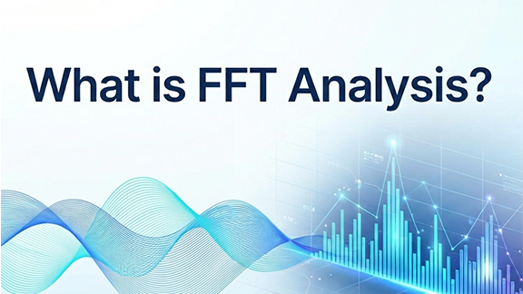
In audio and vibration testing, FFT analysis (Fast Fourier Transform) is one of the tools almost every engineer uses sooner or later: Loudspeaker frequency response Headphone distortion NVH diagnostics Structural resonance troubleshooting Production noise and “mysterious tone” hunting A lot of practical questions are actually asking the same few things: Where is the energy concentrated in frequency? Is it dominated by one tone or a bunch of harmonics? How high is the noise floor? Are there any resonance peaks? FFT is the most universal entry point to answer these questions. This article will help you clarify three things from an engineering perspective: What FFT analysis is How FFT works conceptually How to use FFT correctly and efficiently in practice What Is FFT? In the time domain, a signal is just a waveform changing over time – all components “stacked together” in one trace. You can see it, but it’s hard to tell which frequencies are inside. FFT (Fast Fourier Transform) decomposes a time-domain signal into a sum of sinusoids at different frequencies. In the frequency domain, the signal is represented by frequency + amplitude + phase. In simple terms: Time domain: how the signal moves over time Frequency domain: what frequency components it contains, which are strongest, and how they relate to each other Historically, Fourier’s key idea (early 19th century) was that a complex periodic function can be expressed as a sum of sines and cosines. This evolved into the continuous-time Fourier transform, mapping signals onto a continuous frequency axis. In the computer age, things changed: engineers work with sampled data and typically only have a finite-length record of N samples. That leads to the DFT (Discrete Fourier Transform), which maps N time samples to N discrete frequency bins. FFT (Fast Fourier Transform) is not a different transform. It is a family of algorithms that compute the exact same DFT much more efficiently: Direct DFT: complexity ~ O(N²) FFT: complexity ~ O(N log N) The output X[k] is identical to the DFT result – FFT just gets there far faster by exploiting symmetry and divide-and-conquer. What FFT Is Good at – and What It Isn’t FFT is very good at: Finding deterministic narrowband components Fundamental tones, harmonics, switching frequencies, whistle tones, speed-related lines Looking at broadband distributions Noise floor, 1/f slopes, in-band power, SNR Characterizing system behavior Transfer functions, resonances / anti-resonances, coherence, delay estimation Serving as the foundation of time–frequency analysis STFT, spectrograms, etc. FFT is not good at (or not sufficient on its own for): Strongly non-stationary signals and “instantaneous frequency” For chirps and rapidly changing content, you need STFT, wavelets, or other time–frequency methods, not a single FFT on a long record Separating two extremely close tones below your frequency resolution If the spacing is smaller than your bin resolution (set by N), no algorithm will magically resolve them Turning short data into “long measurements” Zero padding only interpolates the spectrum visually; it does not add new information Before Using FFT: Key Concepts to Get Right To use FFT well, you need to be confident about a few fundamentals: Sampling rate DFT and its interpretation What you actually plot (magnitude, amplitude, power, PSD) Windowing and spectral leakage Averaging Sampling Rate: How High in Frequency You Can See Before FFT, you already made one crucial decision: sampling. A continuous-time signal x(t) is turned into a discrete sequence x[n]=x(n/fs). The sampling rate fsf_sfs​ determines the highest frequency you can observe without aliasing: the Nyquist frequency, fs/2. If the analog signal contains energy above fs/2, it does not disappear – it folds back into the band below Nyquist as aliasing. Once aliasing happens, FFT cannot “undo” it; the information is irretrievably mixed. In practice, you must use an anti-alias filter before the ADC (or before any resampling) to suppress components above Nyquist. Example: A 900 Hz sine sampled at fs=1 kHz will appear at 100 Hz in the discrete spectrum – a classic aliasing artifact. DFT Computation and Interpretation Given N samples x[0]..x[N−1], the DFT is defined as: The inverse transform (IDFT) reconstructs the time signal: Intuitively, X[k] tells you how strongly the signal correlates with a complex exponential at that bin’s frequency. The magnitude X[k] indicates “how much” of that frequency component exists The phase encodes time alignment relative to other components What Are You Plotting? Magnitude, Amplitude, Power, PSD From one set of FFT results X[k], you can create many different “spectra” that look similar but represent different physical quantities. This is where confusion between tools and platforms often arises. Common variants include: Magnitude spectrum |X[k]| Units depend on normalization (e.g., “V·samples”) Useful for locating peaks, harmonics, and general spectral shape Amplitude spectrum Properly scaled magnitude, in physical units (e.g. V) Appropriate for reading off sinusoid amplitudes and doing calibrated measurements Power spectrum |X[k]|² Again, scaling dependent; often used for power/energy comparisons when conventions are fixed Power Spectral Density (PSD) Sxx(f) Units like V²/Hz or Pa²/Hz Used for noise analysis, band power, and comparisons across different FFT lengths If you want to compare noise levels across different FFT sizes, windows, or tools, use PSD (or amplitude spectral density). Raw |X| or  |X|² values are rarely directly comparable. A Concrete Example: Two Tones in Time and Frequency Imagine a signal consisting of two sinusoids at different frequencies. In the time domain, their sum may look like a “wobbly” waveform. In the frequency domain (FFT/PSD), you will see two distinct narrow peaks at the corresponding frequencies. In OpenTest’s FFT analysis, you can visualise both the spectrum and PSD/ASD side by side, making it easy to: Identify tonal components Inspect noise distribution Compare different operating conditions on the same frequency grid Try it yourself: Download the free OpenTest edition and run an FFT on a simple two-tone signal to see both peaks clearly separated. Window Functions and Spectral Leakage: Cleaning Up Spectra In theory, FFT assumes the sampled block contains an integer number of periods and is then repeated periodically. In reality, the record almost never lines up perfectly with an integer number of cycles. When you repeat that block, you get discontinuities at the boundaries, which causes energy to spread into neighboring bins — this is spectral leakage. To reduce leakage, we typically apply a window function to the time record before doing FFT. A window simultaneously affects: Main lobe width Wider main lobe = peaks get broader → it’s harder to separate close tones Side lobe height Lower side lobes = easier to see small peaks near a large one (better dynamic range) Amplitude/energy scaling Windows change the relationship between a pure tone’s true amplitude and the observed peak, as well as the noise floor level Some practical guidelines: Rectangular window Only use when you can ensure coherent sampling (an integer number of periods in the record) and you want the narrowest possible main lobe Hanning (Hann) window A very robust default choice for general acoustics and vibration work Widely used with Welch/PSD methods Hamming Similar to Hann, with slightly different side-lobe behavior, common in communications Blackman / Blackman–Harris Lower side lobes, useful when you need to see small peaks next to big ones, at the cost of a wider main lobe In OpenTest, you can switch between different window functions in the FFT analysis module and immediately see the impact on peak width, side lobes, and noise floor. Averaging: Making Spectra More Stable For noisy or non-stationary signals, a single FFT can look very “spiky” or unstable. By averaging multiple spectra, you obtain a smoother, more repeatable result. Common averaging types include: Linear averaging A simple arithmetic mean of several FFT results Exponential averaging Recent data gets more weight; good for live monitoring when the spectrum should react but not jump wildly Energy (power) averaging Based on power; ensures power-related quantities remain consistent A good averaging configuration strikes a balance between suppressing random fluctuations and preserving genuine changes in the signal. Where Do We Use FFT in Practice? Audio and Acoustics Typical applications include: Finding feedback frequencies, harmonic distortion, and device noise floors Frequency response (transfer function) measurement Room modes / resonance analysis Spectrograms of speech, music, and equipment noise In audio/acoustics, you must be clear about units and conventions: dB SPL, A-weighting, 1/3-octave bands, etc. FFT is the engine; the reporting convention (reference, weighting, bandwidth) must be clearly defined. Vibration and Rotating Machinery Identifying speed-related peaks (1X, 2X, gear mesh frequencies) Structural resonances and mode behavior under different operating conditions Bearing diagnostics, gear whine, imbalance, misalignment For bearing and gearbox analysis, envelope detection/demodulation is often used: Band-pass filter the signal Demodulate and then perform FFT on the envelope to reveal fault frequencies If the rotational speed is changing, a simple FFT will “smear” peaks. In that case, order tracking or synchronous resampling is more appropriate, turning the axis from “frequency” into “order”. Power Electronics and Power Quality Line frequency harmonics (50/60 Hz and multiples), THD, ripple, switching spikes Pre-compliance EMI checks: spectral lines, noise floor, in-band power In power systems, non-coherent sampling is a common issue: if the record length is not an integer number of mains cycles, leakage affects harmonic accuracy. Solutions include synchronous sampling, integer-cycle windows, or specialized harmonic analyzers. RF and Communications (Baseband View) Modulated signal spectra and spectral masks OFDM and multi-carrier spectral analysis, adjacent channel leakage Here, consistency is paramount: Same units Same bandwidth (RBW) Same window, detector, and averaging style FFT itself is straightforward; turning it into comparable power measurements requires tightly defined settings. Imaging and 2D Filtering 2D FFT extends the same idea to images: Edges correspond to high spatial frequencies; smooth areas to low frequencies Low-pass / high-pass filtering, removal of periodic noise, convolution acceleration in the frequency domain The same periodic extension assumption now applies in 2D: discontinuities at image borders produce strong artifacts in the frequency domain. Padding, mirrored borders, or 2D windows are common ways to mitigate this. Turning FFT into an Everyday Engineering Tool From a mathematical standpoint, FFT is not particularly “lightweight”. But in engineering use, the goal is actually simple: See what’s hidden inside the signal more clearly and much faster. When you understand: What FFT really computes How sampling, windowing, scaling, and averaging affect the result When to use spectra vs PSD, and which settings matter for your use case …then FFT stops being an abstract math topic and becomes a practical, everyday tool for acoustics and vibration work – from R&D and validation all the way to production testing. Download and get started now -> or fill out the form below ↓ to schedule a live demo. Explore more features and application stories at www.opentest.com.

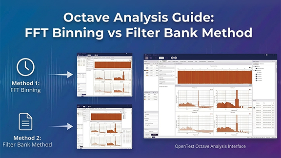
Octave-band analysis can be implemented in two fundamentally different ways: FFT binning (integrating PSD/FFT bins into 1/1- and 1/3-octave bands) and a true octave filter bank (standards-oriented bandpass filters + RMS/Leq averaging). In this post, we compare how the two methods work, where their results match, where they diverge (scaling, window ENBW, band-edge weighting, latency, transient response), and how OpenTest supports both for acoustics, NVH, and compliance measurement. For a detailed explanation of the concepts, read this → Octave-Band Analysis: The Mathematical and Engineering Rationale Octave-band filter banks (true octave / CPB filter bank) Parallel bandpass filters + energy detector + time averaging A filter-bank (true octave) analyzer typically: Design a bandpass filter H_b(z) (or H_b(s)) for each band center frequency. Run filters in parallel to obtain band signals y_b(t). Compute band mean-square/power and apply time averaging to output band levels. To be comparable across instruments, filter magnitude responses must satisfy IEC/ANSI tolerance masks (class) for the specified filter set. [1][3] IIR vs FIR: why IIR (cascaded biquads) is common in practice IIR advantages: lower order for a given roll-off, lower compute, good for real-time/embedded; stable when implemented as SOS/biquads. FIR advantages: linear phase is possible (useful when waveform shape matters); design/verification can be more straightforward. For band-level outputs, phase is usually not the primary concern, so IIR filter banks are common. Multirate processing: the “secret weapon” of CPB filter banks Low-frequency CPB bands are very narrow. Implementing them at the full sampling rate is inefficient. A common strategy is to group bands by octave and downsample for low-frequency groups: Low-pass then decimate (e.g., by 2 per octave) for lower-frequency groups. Implement the corresponding bandpass filters at the reduced sampling rate. Ensure adequate anti-aliasing before decimation. Time averaging / time weighting: band levels are statistics, not instantaneous values Band levels typically require time averaging. Common options include block RMS, exponential averaging, or Leq (energy-equivalent level). In sound level meter contexts, IEC 61672-1 defines Fast/Slow time weightings (Fast ~125 ms, Slow ~1 s). [5][6] Engineering implication: different time constants produce different readings, so time weighting must be stated in reports. How to validate that a filter bank behaves “like the standard” Sine sweep: verify passband behavior and adjacent-band isolation; observe time delay effects. Pink/white noise: verify average band levels and variance/stabilization time; check effective bandwidth behavior. Impulse/step: examine ringing and time response (critical for transient use). Cross-check against a known compliant reference instrument/implementation. From band definitions to compliant digital filters: an end-to-end workflow (conceptual) Choose the band system: base-10/base-2, the fraction 1/b (commonly b=3), generate exact fm and f1/f2. Choose performance target: which standard edition and which class/mask tolerance? Choose filter structure: IIR SOS for real-time; FIR or forward-backward filtering if phase/zero-phase is required. Design each bandpass: map f1/f2 into the digital domain correctly (e.g., pre-warp for bilinear transform). Implement multirate if needed: decimate for low-frequency groups with sufficient anti-alias filtering. Verify: magnitude response vs mask; noise tests for effective bandwidth; sweep/impulse tests for time response. Calibrate and report: units and reference quantities, averaging/time weighting, method details. Time response explained: group delay, ringing, and averaging all shape readings A band-level analyzer is a time-domain system (filter → energy detector → smoother), so readings are governed by multiple time scales: Filter group delay: how late events appear in each band. Filter ringing/decay: how long a short pulse “rings” within a band. Energy averaging/time weighting: the time resolution vs fluctuation of the output level. Thus, for transients (impacts, start/stop events, sweeps), different compliant implementations can yield different peak levels and time tracks—consistent with ANSI’s caution. [3] Rule of thumb: for steady-state contributions, use longer averaging for stability; for transient localization, shorten averaging but accept higher variability and lock down algorithm details. Common real-time pitfalls Forgetting anti-aliasing in the decimation chain: low-frequency bands become contaminated by aliasing. Numerical instability of high-Q low-frequency IIR sections: use SOS/biquads and sufficient precision. Averaging in dB: always average in energy/mean-square, then convert to dB. Assuming band energies must sum exactly to total energy: standard filters are not necessarily power-complementary; verify using standard-consistent criteria instead. Octave-Band Filter Bank Analysis in OpenTest OpenTest supports octave-band analysis using a filter-bank approach:1) Connect the device, such as SonoDAQ Pro2) Select the channels and adjust the parameter settings. For an external microphone, enable IEPE and switch to acoustic signal measurement.3) In the Octave-Band Analysis section under Measurement Mode, choose the IEC 61260-1 algorithm. It supports real-time analysis, linear averaging, exponential averaging, and peak hold.4) After configuring the parameters, click the Test button to start the measurement.5) A single recording can be analyzed simultaneously in 1/1-octave, 1/3-octave, 1/6-octave, 1/12-octave, 1/24-octave, and 1/24-octave bands. Figure 1: Octave-Band Filter Bank Analysis in OpenTest FFT binning and FFT synthesis FFT binning: convert a narrowband spectrum into CPB band integrals Estimate spectrum (single FFT, Welch PSD, or STFT). Integrate/sum within each octave/fractional-octave band to obtain band power. This is common in software/offline work because a single FFT provides high-resolution spectrum that can be re-binned into any band system (1/1, 1/3, 1/12, …). Key challenge #1: FFT scaling and window corrections After an FFT, scaling depends on your definitions: 1/N normalization, amplitude vs power vs PSD, one-sided vs two-sided spectrum, and windowing. For noise measurements, ENBW is crucial; ignoring it can introduce systematic offsets. [7] A practical PSD normalization (periodogram form) # convert to one-sided PSD: multiply by 2 except DC (and Nyquist if present) This yields PSD in units of (input unit)²/Hz and supports energy consistency checks by integrating PSD over frequency. Two quick self-checks for scaling White noise check: generate noise with known variance σ²; integrate one-sided PSD over 0..fs/2 and recover ≈σ² (accounting for the ×2 rule). Pure tone check: generate a sine with amplitude A (RMS=A/√2); integrating spectral energy should recover ≈A²/2 (subject to leakage and window choice). If both checks pass, your FFT scaling is likely correct; then partial-bin weighting and octave binning become meaningful. Key challenge #2: band edges rarely align to bins → partial-bin weighting Hard include/exclude decisions at band edges cause step-like errors, especially at low frequency where bands are narrow. Use overlap-based weighting (Section 4.2.4) for the boundary bins. Does zero-padding solve edge misalignment? (common misconception) Zero-padding interpolates the displayed spectrum but does not improve true frequency resolution (which is set by the original window length). It can reduce visual stair-stepping but cannot turn 1–2-bin low-frequency bands into reliable band-level estimates. Fundamental fixes are longer windows or multirate processing/filter banks. Key challenge #3: time–frequency trade-off (window length sets low-frequency accuracy and delay) FFT resolution is Δf = fs/N. Low-frequency 1/3-octave bands can be only a few Hz wide, so achieving enough bins per band requires very large N, increasing latency and smoothing transients. Root cause: 1/3 octave is constant-Q, but STFT uses constant-Δf bins In CPB, band width scales with frequency (Δf_band ∝ f, constant-Q). In STFT, bin spacing is constant (Δf_bin constant). Therefore low-frequency CPB needs extremely fine Δf_bin (long windows), while high frequency is over-resolved. Solution routes: long-window STFT vs multirate STFT vs CQT/wavelets Long-window STFT: simplest, but high latency and transient smearing. Multirate STFT: downsample low-frequency content and FFT at lower fs, similar in spirit to multirate filter banks. Constant-Q transform (CQT) / wavelets: naturally logarithmic resolution, but matching IEC/ANSI masks requires extra calibration/validation. [4] For compliance measurements, standards-oriented filter banks are preferred; for research/feature extraction, CQT/wavelets can be attractive. FFT synthesis: constructing per-band filtering in the frequency domain FFT synthesis pushes the FFT approach closer to a filter bank: Define a frequency-domain weight W_b[k] per band (brick-wall or smooth/mask-like). Compute Y_b[k] = X[k]·W_b[k] and IFFT to get y_b[n]. Compute band RMS/averages from y_b[n]. It can easily implement zero-phase (non-causal) filtering. For strict IEC/ANSI matching, W_b and normalization must be carefully designed and validated. Making FFT synthesis stream-like: OLA, dual windows, and amplitude normalization To output continuous time signals per band, use overlap-add (OLA): frame, window, FFT, apply W_b, IFFT, synthesis window, and OLA. Choose analysis/synthesis windows to satisfy COLA (constant overlap-add) conditions (e.g., Hann with 50% overlap) to avoid periodic level modulation. If the goal is to match standard filters, how should W_b be chosen? W_b[k] depends on what you want to match: Match brick-wall integration: W_b is hard 0/1 within [f1,f2]. Match IEC/ANSI filter behavior: |W_b(f)| approximates the standard mask and effective bandwidth (matches ∫|W_b|²). Match energy complementarity for reconstruction: design Σ_b |W_b(f)|² ≈ 1 (Section 7.6). You typically cannot satisfy all three perfectly at once; define your priority (compliance vs decomposition/reconstruction) up front. Energy-conserving frequency-domain filter banks: why Σ|W_b|² matters If you want band energies to sum to total energy (within numerical error), a common design aims for approximate power complementarity: IEC/ANSI masks do not necessarily enforce strict complementarity, so don’t assume exact additivity in compliance contexts. Welch/averaging strategies: how to make FFT band levels stable Use Welch averaging (segment, window, overlap, average power spectra). Average in the power domain (|X|² or PSD), then convert to dB. For non-stationary signals, consider STFT to obtain time–band matrices. Report window type, overlap, averaging count, and ENBW/CG treatment. FFT-Binning Analysis in OpenTest OpenTest supports octave-band analysis based on FFT binning:1) Connect the device, such asSonoDAQ Pro2) Select the channels and adjust the parameter settings. For an external microphone, enable IEPE and switch to acoustic signal measurement.3) In the Octave-Band Analysis section under Measurement Mode, choose the FFT-based algorithm.4) A single recording can be analyzed simultaneously in 1/1-octave, 1/3-octave, 1/6-octave, 1/12-octave, and 1/24-octave bands. Figure 2: FFT-Binning Octave-Band Analysis in OpenTest Filter-bank vs FFT/FFT synthesis: differences, equivalence conditions, and trade-offs A comparison table DimensionFilter-bank (True Octave / CPB)FFT binning / FFT synthesisStandards complianceEasier to match IEC/ANSI magnitude masks; mainstream for hardware instruments. [1][3]Hard binning behaves like band integration; matching masks requires extra weighting or standard-compliant digital filters.Real-time / latencyCausal real-time possible; latency set by filter order and averaging.Block processing adds at least one window length of delay; low-frequency resolution often forces longer windows.Transient responseContinuous output but affected by group delay/ringing; different compliant implementations may differ. [3]Set by STFT windowing; transients are smeared by windows and sensitive to window type/length.Leakage & correctionsControlled via filter design; leakage can be managed.Strongly depends on window and ENBW/scaling; edge-bin misalignment needs partial weighting. [7]InterpretabilityRMS after bandpass filtering—aligned with sound level meters and analyzers.Spectrum estimation + binning—more statistical; interpretation depends on window/averaging settings.ComputationMany filters in parallel; multirate can reduce cost.One FFT can serve all bands; efficient for offline/batch.Phase & reconstructionIIR is typically nonlinear phase (fine for levels).Frequency weights can be zero-phase; reconstruction needs attention to complementarity and transitions. When do both methods give (almost) the same answers? Band-averaged results typically agree closely when: You compare averaged band levels (not transient peak tracks). The signal is approximately stationary and the observation time is long enough. FFT resolution is fine enough that each band contains enough bins (especially at the lowest band). FFT scaling is correct (one-sided handling, Δf, window U, ENBW/CG where needed). Partial-bin weighting is used at band edges. Why differences grow for transients and short events Differences are driven by mismatched time scales: filter banks have band-dependent group delay and ringing but continuous output; STFT uses a fixed window that sets both frequency resolution and time smoothing. If event duration is comparable to the window length or filter impulse response, results depend strongly on implementation details. Error budget: where mismatches usually come from (and how to locate them quickly) Wrong averaging/combination in dB: must average and sum in the energy domain. Inconsistent FFT scaling: 1/N conventions, one-sided vs two-sided, Δf, window normalization U. Missing window corrections: ENBW for noise; coherent gain/leakage for tones. Using nominal frequencies to compute edges instead of exact definitions. No partial-bin weighting at band boundaries (especially harmful at low frequency). Multirate/anti-alias issues in filter banks. Different averaging time constants/windows between methods. True method differences: brick-wall binning vs standard filter skirts/roll-off imply systematic offsets. A strong debugging approach: first match total mean-square using white noise (scaling/ENBW/partial-bin), then validate band centers and adjacent-band isolation using swept sines or tones. Engineering checklist: make 1/3-octave analysis correct, stable, and reproducible Choose a method: compliance → filter bank; offline statistics → FFT binning For regulations/type testing/instrument comparability: prefer IEC/ANSI-compliant filter banks and report standard edition and class. [1][3] For offline processing, large datasets, or flexible band definitions: FFT binning can be efficient, but scaling and boundary weighting must be rigorous. If you need per-band time-domain signals (modulation, envelope, etc.): consider FFT synthesis or explicit filter banks. Selecting FFT parameters from the lowest band (example) Example: fs=48 kHz, lowest band of interest is 20 Hz (1/3 octave). Its bandwidth is only a few Hz. If you want at least M=10 bins per band, you may need Δf_bin ≤ bandwidth/10, implying a very large N (e.g., ~100k points; 2^17=131072). This illustrates why real-time compliance often favors filter banks. Typical mistakes that prevent results from matching Summing magnitude |X| instead of power |X|² or PSD. Averaging in dB instead of in linear power/mean-square. Ignoring ENBW/window scaling for noise. [7] Computing band edges from nominal frequencies. Not stating time weighting/averaging conventions (Fast/Slow/Leq). [5][6] Recommended validation flow (regardless of implementation) Tone-at-center test (or sweep): verify that energy peaks in the correct band and adjacent-band rejection behaves as expected. White/pink noise: verify expected spectral shape in band levels and assess stability/averaging time. Cross-implementation comparison: compare your implementation with a known reference on identical signals; isolate scaling vs definition vs filter-skirt differences. Record and freeze parameters (band definition, windowing, averaging) in the test report. Reproducibility checklist: include these in reports so others can recompute your levels Band definition: base-10 or base-2? b in 1/b? exact vs nominal used for computation? reference frequency fr? Implementation: standard filter bank (IIR/FIR, multirate) vs FFT binning/synthesis; software/library versions. Sampling/preprocessing: fs, detrending/DC removal, anti-alias filtering, resampling. Time averaging: Leq / block RMS / exponential; time constants, block size, overlap, averaging frames; Fast/Slow context if relevant. FFT details (if used): window type, N, hop, zero-padding, PSD normalization, one-sided handling, ENBW/CG, partial-bin weighting. Calibration/units: input units and reference quantities (e.g., 20 µPa), sensor calibration factors and dates. Output definition: RMS vs peak vs band power; 10log vs 20log conventions; any band aggregation steps. If you remember one line: document “band definition + time averaging + FFT scaling/window treatment (if any)”. Most disputes disappear. Quick formulas and numeric example (ready for code/report) Base-10 one-third-octave constants G = 10^(3/10) ≈ 1.995262 r = 10^(1/10) ≈ 1.258925 # adjacent center-frequency ratio k = 10^(1/20) ≈ 1.122018 # edge multiplier about center f1 = fm / k f2 = fm * k Example: the 1 kHz one-third-octave band fm = 1000 Hz f1 = 1000 / 1.122018 ≈ 891.25 Hz f2 = 1000 * 1.122018 ≈ 1122.02 Hz Δf ≈ 230.77 Hz Q ≈ 4.33 OpenTest integrates both methods. Download and get started now -> or fill out the form below ↓ to schedule a live demo. Explore more features and application stories at www.opentest.com. References [1] IEC 61260-1:2014 PDF sample (iTeh): https://cdn.standards.iteh.ai/samples/13383/3c4ae3e762b540cc8111744cb8f0ae8e/IEC-61260-1-2014.pdf [3] ANSI S1.11-2004 preview PDF (ASA/ANSI): https://webstore.ansi.org/preview-pages/ASA/preview_ANSI%2BS1.11-2004.pdf [4] HEAD acoustics Application Note: FFT - 1/n-Octave Analysis - Wavelet (filter bank description): https://cdn.head-acoustics.com/fileadmin/data/global/Application-Notes/SVP/FFT-nthOctave-Wavelet_e.pdf [5] IEC 61672-1:2013 (IEC page): https://webstore.iec.ch/en/publication/5708 [6] NTi Audio Know-how: Fast/Slow time weighting (IEC 61672-1 context): https://www.nti-audio.com/en/support/know-how/fast-slow-impulse-time-weighting-what-do-they-mean [7] MathWorks: ENBW definition example: https://www.mathworks.com/help/signal/ref/enbw.html

Octave-band analysis converts detailed spectra into standardized 1/1- and 1/3-octave bands using constant-percentage bandwidth on a logarithmic frequency axis. In this post, we explain the mathematical basis of CPB, why IEC 61260-1 and ANSI S1.11 define octave bands the way they do, and how band levels are computed in practice (FFT binning vs. filter-bank RMS). The goal: repeatable, comparable results for acoustics, NVH, and compliance measurements. What is octave-band analysis, and what problem does it solve? Octave-band analysis is a family of spectrum analysis methods that partition the frequency axis on a logarithmic scale into band-pass bands. Each band has a constant ratio between its upper and lower cut-off frequencies (constant percentage bandwidth, CPB). Within each band we ignore fine line-spectrum details and focus on total energy / RMS (or power) in that band. In other words, it is not “what happens at every 1 Hz,” but “how energy is distributed across equal relative bandwidths.” This representation naturally matches human hearing and many engineering systems, whose frequency resolution is often closer to a relative (log) scale than a fixed-Hz scale. It is a common reporting format required by many standards: room acoustics parameters, sound insulation ratings, environmental noise, machinery noise, wind/road noise, etc., often use 1/3-octave bands. From linear Hz to log frequency: why CPB looks more like an engineering language Using equal-width frequency bins (e.g., every 10 Hz) to accumulate energy leads to inconsistent behavior across the spectrum: At low frequencies, a 10 Hz bin may be too wide and can smear details. At high frequencies, a 10 Hz bin may be too narrow, giving higher variance and less stable estimates for random noise. In contrast, CPB bandwidth grows with frequency (Δf ∝ f). Each band covers a similar relative change, improving stability and repeatability—important for standardized testing. A visual intuition: bandwidth increases on a linear axis, but is uniform on a log axis Figure 1: the same 1/3-octave bands plotted on a linear frequency axis—bandwidth appears larger at high frequencies Each horizontal segment represents a 1/3-octave band [f1, f2]; the short vertical mark is the band center frequency fm. On a linear axis, higher-frequency bands look wider. Figure 2: the same bands on a logarithmic frequency axis—bands become evenly spaced (the essence of CPB) Once the horizontal axis is logarithmic, these bands appear equal-width/equal-spacing; this is exactly what “constant percentage bandwidth” means. These two figures capture the core idea: octave-band analysis uses equal steps on a log-frequency scale, not equal steps in Hz. Standards and terminology: what do IEC/ANSI/ISO systems actually specify? In practice, “doing 1/3-octave analysis” is constrained by more than just band edges. Standards specify (or strongly imply): how center frequencies are defined (exact vs nominal), the octave ratio definition (base-10 vs base-2), filter tolerances/classes, and even the measurement/averaging conventions used to form band levels. IEC 61260-1:2014 highlights: base-10 ratio, reference frequency, and center-frequency formulas IEC 61260-1:2014 is a key specification for octave-band and fractional-octave-band filters. It adopts a base-10 design: the octave frequency ratio is G = 10^(3/10) ≈ 1.99526 (very close to 2, but not exactly 2). The reference frequency is fr = 1000 Hz. It provides formulas for the exact mid-band (center) frequencies and specifies that the geometric mean of band-edge frequencies equals the center frequency. [1] Key formulas (rearranged from the standard): [1] If the fractional denominator b is odd (e.g., 1, 3, 5, ...): If b is even (e.g., 2, 4, 6, ...): And always: Why does the even-b case look “half-step shifted”? Intuitively, the center-frequency grid is evenly spaced on log(f). When b is even, IEC chooses a half-step offset relative to fr so that band edges align more neatly in common reporting conventions. In practice, a robust implementation is to generate the exact fm sequence using the standard’s formula, then compute edges via f1 = fm / G^(1/(2b)) and f2 = fm * G^(1/(2b)), and only then label bands by the usual nominal frequencies. View the data with OpenTest (IEC 61260-1 Octave-Band Analysis) -> Band edges, center frequency, and the bandwidth designator b Standards commonly use 1/b as the “bandwidth designator”: 1/1 is one octave, 1/3 is one-third octave, etc. [1] Once (G, b, fr) are chosen, the entire band set (centers and edges) is fixed mathematically. Exact vs nominal: why two “center frequencies” appear for the same band “Exact” center frequencies are used for mathematically consistent definitions and filter design; “nominal” values are used for labeling and reporting. [1] ISO 266:1997 defines preferred frequencies for acoustics measurements based on ISO 3 preferred-number series (R10), referenced to 1000 Hz. [2] As a result, the exact geometric sequence is typically labeled with familiar nominal values such as: 20, 25, 31.5, 40, 50, 63, 80, 100, 125, 160, …, 1k, 1.25k, 1.6k, 2k, 2.5k, 3.15k, …, 20k. Implementation tip: compute edges from exact frequencies; only round/display as nominal. This avoids drifting away from the standard. Base-10 vs base-2: why standards don’t insist on an exact 2:1 octave Although “octave” is often thought of as 2:1, IEC 61260-1 specifies base-10 (G=10^(3/10)) rather than G=2. Key motivations include: Alignment with decimal preferred-number series (ISO 266 is tied to R10). [2] International consistency: IEC 61260-1:2014 specifies base-10 and notes that base-2 designs are less likely to remain compliant far from the reference frequency. [1] In base-10, one-third octave corresponds to 10^(1/10) ≈ 1.258925 (also interpretable as 1/10 decade), which yields a clean mapping: 10 one-third-octave bands per decade. “10 one-third-octave bands = 1 decade”: why this matters With base-10 one-third-octave spacing, each step multiplies frequency by r = 10^(1/10). Therefore: 10 consecutive 1/3-octave bands multiply frequency by exactly 10 (one decade). This matches ISO 266/R10 conventions and simplifies tables, plotting, and communication. Standardization values readability and consistency as much as raw mathematical purity. Figure 3: Base-10 one-third-octave spacing—10 equal ratio steps per decade (×10 in frequency) ANSI S1.11 / ANSI/ASA S1.11: tolerance classes and a transient-signal caution ANSI S1.11 (and later ANSI/ASA adoptions aligned with IEC 61260-1) specify performance requirements for filter sets and analyzers, including tolerance classes (often class 0/1/2 depending on edition). [3][4] A practical caution in ANSI documents: for transient signals, different compliant implementations can produce different results. [3] This highlights that time response (group delay, ringing, averaging time constants) matters for transient analysis. What do class/mask/effective bandwidth actually control? “I used 1/3-octave bands” is not just about nominal band edges. Standards aim to ensure different instruments/algorithms yield comparable results by constraining: Frequency spacing: center-frequency sequence and edge definitions (base-10, exact/nominal, f1/f2). Magnitude response tolerance (mask): allowable ripple near passband and required attenuation away from center. Energy consistency for broadband noise: constraints on effective bandwidth so band levels are comparable across implementations. Effective bandwidth matters because real filters are not ideal brick walls. For broadband noise, the output energy depends on ∫|H(f)|^2 S(f)df. Differences in passband ripple, skirts, and roll-off can cause systematic offsets. Standards constrain effective bandwidth to keep such offsets within acceptable limits. [1][3][4] The transient caution is not a contradiction: masks mainly constrain steady-state frequency-domain behavior, while transients depend on phase/group delay, ringing, and time averaging. [3] Mathematics: band definitions, bandwidth, Q, and band indexing CPB and equal spacing on a log axis CPB is equivalent to equal-width spacing in log-frequency. If u = log(f), then every band spans a fixed Δu. Many spectra (e.g., 1/f-type) look smoother and statistically more stable in log frequency. Band-edge formulas from the geometric-mean definition (general 1/b form) IEC defines the center frequency as the geometric mean of the edges: fm = sqrt(f1 f2). [1] For 1/b octave bands, the edge ratio is typically f2/f1 = G^(1/b), where G is the octave ratio. Then: For base-10 one-third octave (b=3): G=10^(3/10). Adjacent center ratio is r = G^(1/3) = 10^(1/10) ≈ 1.258925; edge multiplier is k = 10^(1/20) ≈ 1.122018. Q-factor and resolution: octave analysis is constant-Q analysis Define Q = fm / (f2 − f1). For CPB bands, Δf = f2 − f1 scales with fm, so Q depends only on b and G (not on frequency). Quick reference (base-10, fr=1000 Hz): Fractional-octaveBand ratio f2/f1Relative bandwidth Δf/fmQ = fm/Δf1/11.9952620.7045921.4191/21.4125380.3471072.8811/31.2589250.2307684.3331/61.1220180.1151938.6811/121.0592540.05757317.369 Interpretation: for 1/3 octave, Q≈4.33 and each band is about 23% wide relative to its center. Finer bands (1/6, 1/12) give higher resolution but higher variance for random noise and typically require longer averaging. Band numbering (integer index) and formulaic enumeration Implementations often use an integer band index x. In IEC, x appears directly in the center-frequency formula: fm = fr * G^(x/b). [1] This provides a stable way to enumerate all bands covering a target frequency range and ensures contiguous, standard-consistent edges. For base-10: so and you can invert as Figure 4: Q factor for common fractional-octave bandwidths (base-10 definition) Two meanings of “1/3 octave”: base-2 vs base-10—do not mix them Some literature uses base-2: adjacent centers are 2^(1/3). IEC 61260-1 and much modern acoustics practice use base-10: adjacent centers are 10^(1/10). A quick check: if nominal centers look like 1.0k → 1.25k → 1.6k → 2.0k (R10 style), it is likely base-10. Mathematical definition of band levels: from PSD integration to dB reporting Continuous-frequency view: integrate PSD within the band Octave-band level is essentially the integral of power spectral density over a frequency band. For sound pressure p(t): For vibration (velocity/acceleration), the same logic applies with different units and reference quantities. Key point: because dB is logarithmic, any summation or averaging must be performed in the linear power/mean-square domain first. Two discrete implementations: filter-bank RMS vs FFT/PSD binning Filter-bank method: y_b(t)=BandPass_b{x(t)}, then compute mean(y_b^2) as band mean-square (optionally with time averaging). FFT/PSD binning method: estimate S_pp(f) (e.g., via periodogram/Welch), then numerically integrate/sum bins within [f1,f2]. For long, stationary signals, averaged results can be very close. For transients, sweeps, and short events, they often differ. Be explicit about what spectrum you have: magnitude, power, PSD (and dB/Hz) Magnitude spectrum |X(f)|: amplitude units (e.g., Pa), useful for tones/harmonics. Power spectrum |X(f)|²: mean-square units (Pa²). Power spectral density (PSD): mean-square per Hz (Pa²/Hz), most common for noise. Because octave-band levels represent band mean-square/power, you must end up integrating/summing in Pa² (or analogous) regardless of starting representation. Frequency resolution and one-sided spectra: Δf, 0..fs/2, and the “×2” rule FFT bin spacing is Δf = fs/N. A typical discrete approximation is: If you use a one-sided spectrum (0..fs/2), to conserve energy you typically multiply all non-DC and non-Nyquist bins by 2 (because negative-frequency power is folded into the positive side). Different software handles these conventions differently, so align definitions before comparing results. Window corrections: coherent gain (tones) vs ENBW (noise) are different Windowing reduces spectral leakage but changes scaling: For tone amplitude: correct by coherent gain (CG), often CG = sum(w)/N. For broadband noise/PSD: correct by equivalent noise bandwidth (ENBW), e.g., ENBW = fs·sum(w²)/(sum(w))². [9] CG controls peak amplitude; ENBW controls average noise-floor area. Octave-band levels are energy statistics and are more sensitive to ENBW. WindowCoherent Gain (CG)ENBW (bins)Rectangular1.0001.000Hann0.5001.500Hamming0.5401.363Blackman0.4201.727 Partial-bin weighting: what to do when band edges do not align to FFT bins Band edges rarely land exactly on bin frequencies. Treat PSD as approximately constant within each bin of width Δf, and weight boundary bins by their overlap fraction: This produces smoother, more physically consistent band levels when N or band edges change. Figure 5: Partial-bin weighting schematic when band edges do not align with FFT bins A unifying formula: both methods compute ∫|H_b(f)|² S_xx(f) df Both filter-bank and PSD binning can be written as: Brick-wall binning corresponds to |H_b|² being 1 inside [f1,f2] and 0 outside. A true standards-compliant filter has a roll-off and ripple, which is why standards constrain masks and effective bandwidth. Band aggregation: composing 1-octave from 1/3-octave, and forming total levels Under ideal partitioning and energy accounting: Three adjacent 1/3-octave bands can be combined to approximate one full octave band. Summing all band energies over a covered range yields the total energy. Always combine in the energy domain. If L_i are band levels in dB, energies are E_i = 10^(L_i/10). Then: IEC 61260-1 notes that fractional-octave results can be combined to form wider-band levels. [1] Effective bandwidth: why standards specify it Real filters are not ideal rectangles. For white noise (constant PSD S0), output mean-square is: For non-white spectra such as pink noise (PSD ~ 1/f), standards may define normalized effective bandwidth with weighting to maintain comparability across typical engineering noise spectra. [1] Practical implication: FFT “hard-binning” implicitly assumes a brick-wall filter with B_eff = (f2 − f1). A compliant octave filter has skirts, so B_eff can differ slightly (and by class). To match results, either approximate the standard’s |H(f)|² in the frequency domain or document the methodological difference. Why 1/3 octave is favored (math + perception + engineering trade-offs) Information density is “just right”: finer than 1 octave, steadier than very fine fractions A single octave band can be too coarse and hide spectral shape; very fine fractions (e.g., 1/12, 1/24) can be unstable and expensive: Higher estimator variance for random noise (each band captures less energy). More computation and higher reporting burden. Often more detail than regulations or rating schemes need. One-third octave is the classic compromise: enough resolution for engineering insight, stable enough for standardized measurements, and broadly supported by instruments and software. Psychoacoustics: critical bands in mid-frequencies are close to 1/3 octave Many psychoacoustics references describe ~24 critical bands across the audible range, and in the mid-frequency region the critical-bandwidth is often similar to a 1/3-octave bandwidth. [7][8] This makes 1/3 octave a natural intermediate representation for problems tied to perceived sound, while still being more standardized than Bark/ERB scales. Direct standards/application pull: many workflows mandate 1/3 octave I/O Once major standards define inputs/outputs in 1/3 octave, ecosystems (instruments, software, reporting templates) converge around it. Examples: Building acoustics ratings: ISO 717-1 references one-third-octave bands for single-number quantity calculations. [5] Room acoustics parameters (e.g., reverberation time) are commonly reported in octave/one-third-octave bands (ISO 3382 series). [6] Extra base-10 benefits: R10 tables, 10 bands/decade, readability 10 bands per decade: multiplying frequency by 10 corresponds to exactly 10 one-third-octave steps (very clean for log plots). R10 preferred numbers: 1.00, 1.25, 1.60, 2.00, 2.50, 3.15, 4.00, 5.00, 6.30, 8.00 (×10^n) are widely recognized and easy to communicate. Compared with base-2, decimal labeling is less awkward and cross-standard ambiguity is reduced. Octave-band analysis is typically implemented using either FFT binning or a filter bank. Keep reading -> Octave-Band Analysis Guide: FFT Binning vs. Filter Bank OpenTest integrates both methods. Download and get started now -> or fill out the form below ↓ to schedule a live demo. Explore more features and application stories at www.opentest.com. References [1] IEC 61260-1:2014 PDF sample (iTeh): https://cdn.standards.iteh.ai/samples/13383/3c4ae3e762b540cc8111744cb8f0ae8e/IEC-61260-1-2014.pdf [2] ISO 266:1997, Acoustics - Preferred frequencies (ISO): https://www.iso.org/obp/ui/ [3] ANSI S1.11-2004 preview PDF (ASA/ANSI): https://webstore.ansi.org/preview-pages/ASA/preview_ANSI%2BS1.11-2004.pdf [4] ANSI/ASA S1.11-2014/Part 1 / IEC 61260-1:2014 preview: https://webstore.ansi.org/preview-pages/ASA/preview_ANSI%2BASA%2BS1.11-2014%2BPart%2B1%2BIEC%2B61260-1-2014%2B%28R2019%29.pdf [5] ISO 717-1:2020 abstract (mentions one-third-octave usage): https://www.iso.org/standard/77435.html [6] ISO 3382-2:2008 abstract (room acoustics parameters): https://www.iso.org/standard/36201.html [7] Ansys Help: Bark scale and critical bands (mentions midrange close to third octave): https://ansyshelp.ansys.com/public/Views/Secured/corp/v252/en/Sound_SAS_UG/Sound/UG_SAS/bark_scale_and_critical_bands_179506.html [8] Simon Fraser University Sonic Studio Handbook: Critical Band and Critical Bandwidth: https://www.sfu.ca/sonic-studio-webdav/cmns/Handbook5/handbook/Critical_Band.html [9] MathWorks: ENBW definition example: https://www.mathworks.com/help/signal/ref/enbw.html

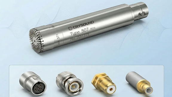
From the outside, a measurement microphone looks deceptively simple. But in real-world engineering, its interface options are surprisingly diverse: Lemo, BNC, Microdot, 10-32 UNF, M5, SMB… Many newcomers to acoustics ask questions like: Why can’t microphone interfaces be standardized? Why are cables often not interchangeable between microphones? What power and signal schemes are hidden behind different connectors? This article provides a structured overview of common measurement microphone interfaces, looking at physical connectors, powering methods, cable characteristics, and typical application-driven selection. Main Physical Interfaces for Measurement Microphones Below is a connector-by-connector summary, including the typical powering approach for each. Lemo (5-pin, 7-pin): The Classic Solution for Externally Polarized Microphones Lemo is a precision circular multi-pin connector and is the most common choice for externally polarized measurement microphones. The Lemo B series is widely used (e.g., 0B, 1B, 2B), and most standard measurement microphones adopt the Lemo 1B interface. Key Characteristics A multi-pin connector can carry multiple signals simultaneously, such as: Microphone output (analog signal) External polarization high voltage (typically 200 V) Preamplifier power supply Calibration/identification signals Additional benefits: Very reliable mechanical locking Well-suited for lab environments, metrology, and semi-anechoic chamber measurements where stability and traceability matter Notes on External Polarization Common polarization voltage is 200 V; some systems support switching between 0 V / 200 V Polarization voltage stability affects microphone sensitivity; in engineering practice, sensitivity variation is often treated as approximately proportional to voltage variation The preamplifier is typically powered separately (up to 120 V) but delivered via the same multi-pin connector Maximum output voltage can reach 50 Vp Includes pins for charge injection methods Separate output and ground paths help achieve lower noise In metrology labs, type testing, acoustic calibration, and high-precision semi-anechoic chamber work, the combination of “externally polarized microphone + Lemo multi-pin connector” is essentially a standard configuration. When not to use Lemo: Harsh environments with heavy contamination, oil exposure, and salt spray High costs of cables and connectors require careful trade-offs in field engineering applications BNC: The Most Common External Connector for IEPE Microphones Names like IEPE / ICP / CCP refer to the same general technology route: constant-current powering, where power and signal are transmitted on the same line (Constant Current Powering). In this system, the most common physical connector is the coaxial BNC. Interface and Powering Characteristics Coaxial structure, ideal for analog voltage transmission Bayonet lock (quick and reliable plug/unplug) Supports longer cable runs with good noise immunity Low cost and highly universal Typical IEPE Powering Parameters Constant current: 2–20 mA (common settings include 2 mA, 4 mA, 8 mA, etc.) Compliance voltage (supply capability): typically 18–24 V Maximum output voltage: generally around 8 Vp If the constant current is too low or the compliance voltage is insufficient, the maximum output signal swing is limited—directly affecting the maximum measurable SPL and the linear measurement range. In everyday testing such as engineering noise measurements, NVH, and environmental noise work, “IEPE microphone + BNC” has become the de facto standard. When not to use BNC: Applications requiring long-distance transmission of high-frequency signals, where signal attenuation becomes significant Applications involving frequent plugging and unplugging, to avoid an increased risk of poor electrical contact Microdot (10-32 UNF / M5): Lightweight Connectivity for Small Microphones Microdot is a threaded miniature coax connector widely used for small sensors (compact measurement microphones, accelerometers, etc.). It commonly uses a 10-32 UNF thread. What “10-32 UNF” Really Means This is simply an imperial fine-thread standard: Nominal diameter: 0.19 inch ≈ 4.826 mm Pitch: 1/32 inch ≈ 0.7938 mm Because 10-32 UNF is the typical thread used on Microdot connectors, the term “10-32 UNF” is often used informally to refer to the Microdot interface itself. What about M5? M5 is a metric thread standard: Nominal diameter: 5 mm Pitch: 0.8 mm Its dimensions are close to 10-32 UNF, and when tolerances are not extremely strict it can serve as a substitute—commonly seen in accelerometers or vibration microphones. Interface Characteristics Very compact; ideal for lightweight setups Threaded locking provides strong mechanical stability Commonly paired with IEPE powering Best for short runs and high-speed signal transmission When microphones must be placed in tight spaces, or where sensor mass/size is critical, Microdot is a common choice for compact, high-density installations. When not to use Microdot: Applications requiring quick connect/disconnect or frequent sensor replacement Use in systems with low constraints on installation space and requiring large-size connectors or high-power transmission, to avoid increased connection complexity and cost SMB (SubMiniature B): For High-Density Multi-Channel or Internal Connections SMB is a small “push-on” coaxial connector. Interface Characteristics Compact size supports high channel density Push-on structure enables fast connection Better high-frequency performance than BNC More suitable for semi-permanent internal wiring SMB is often best viewed as an engineering connector used inside equipment, rather than a field-plugging standard. When not to use Microdot: Applications involving frequent plugging and unplugging or repeated mechanical stress Use as a front-end connection interface for external devices, to avoid structural damage and reduced reliability Extended Interface Function: TEDS and Smart Identification In multi-channel and integrated systems, TEDS (Transducer Electronic Data Sheet) is increasingly common. By integrating a small memory chip into the sensor or cable, TEDS can store: Model and serial number Sensitivity Calibration date and other parameters Compatible front-end hardware or acquisition software can automatically read TEDS to: Identify the sensor type on each channel Load sensitivity and calibration coefficients automatically Reduce manual entry errors Save calibration time and labor At the connector level, TEDS is typically implemented by using certain pins in multi-pin Lemo connectors, or via overlay methods in specific BNC-based solutions. When planning an interface system, it’s wise to consider early on whether TEDS support is required. Why Are There So Many Interfaces? Connector diversity is best explained from three perspectives: Different Polarization and Powering Schemes Externally polarized microphones (≈ 200 V polarization) → better suited to multi-pin connectors like Lemo Prepolarized + IEPE systems → better suited to coaxial connectors like BNC / Microdot / SMB Different Scenarios and Priorities Laboratory / metrology: high stability, multiple signals in one cable, secure locking → Lemo Field engineering / environmental measurement: convenient wiring, strong universality → BNC + IEPE Miniaturization / high-density arrays: size and channel density first → Microdot / SMB Long Product Lifecycles and Backward Compatibility Measurement systems often have lifecycles of 10–20 years or more To avoid forcing users to replace large numbers of cables and front-end systems, manufacturers typically continue existing interface ecosystems Under long lifecycle constraints, “full unification” is often impractical and offers limited engineering return Typical Application Mapping (Quick Reference) Engineering noise, NVH, vibration/noise tests: BNC / MicrodotEasy wiring, many channels, low maintenance cost Precision lab measurement, type testing, metrology calibration: Lemo 7-pin / 5-pinSupports polarization HV and multiple signals; suitable for traceable high-precision measurement Acoustic arrays, multi-channel acquisition card systems: Microdot / SMBHigh channel density, compact wiring, easier system integration Long-term environmental noise monitoring systems: BNC / customized protected connectorsFocus on weather resistance, waterproofing, salt fog resistance, and stable long-distance transmission Conclusion The variety of measurement microphone interfaces is mainly the result of trade-offs between technology routes, application requirements, and historical compatibility—not simply a “lack of standards”. Taking NVH testing as an example: if an existing system uses BNC connectors to connect accelerometers, high-frequency signal attenuation and intermittent contact issues may occur in multi-channel array measurements. To improve connection reliability and signal quality, LEMO connectors with locking mechanisms and superior vibration resistance should be selected. After replacement, signal transmission stability is significantly improved, noise interference is reduced, and the consistency of test data is enhanced. You are welcome to learn more about microphone functions and hardware solutions on our website and use the “Get in touch” form to contact the CRYSOUND team.